
Adaptrade Software Newsletter Article
Deep Neural Networks for Price Prediction, Part 1
Ever since a deep convolutional neural network set a new record in the ImageNet image classification contest back in 2012,1 deep neural networks have revolutionized the field of artificial intelligence. Now, of course, almost everyone is familiar with large language models (LLMs), such as ChatGPT, which are based on deep neural networks. However, far less attention has been paid to the use of similar technologies for predicting financial market prices.
With this article and the next one, I'll preview a new feature I've been working on for my trading strategy generator, Adaptrade Builder, that allows the user to train and use a deep neural network for predicting market prices. In this article, I'll cover the basic concepts involved and illustrate the potential of deep neural networks by training several networks on different price series. In the next article (Part 2), I'll show how these networks can be used as part of a trading strategy.
Why Deep Neural Networks?
Developing a systematic trading strategy is about finding an edge in the market and turning that into code. Oftentimes, that means finding some mix of indicators and price patterns that when used in combination with specific entry and exit orders results in an overall net profit in out-of-sample testing. Strictly speaking, a trading strategy is not about predicting future prices. In fact, even with less than 50% winners — sometimes much less — a strategy can still be profitable if it has a high win/loss ratio. Nonetheless, if we had a way to predict the next day's price (or the price in two days, next week, etc.) with any reasonable accuracy, that would certainly be an advantage.
That's where deep neural networks (DNNs) come in. DNNs are powerful general-purpose function approximators, which gives them an advantage over older machine learning methods and other, simpler techniques that have been used to predict market prices. By adding more "nodes" to the neural network, a DNN can be made as complex as needed to capture the market's essential dynamics. And unlike traditional systematic trading methods, neural networks are less likely to overfit the training data, even when there are many more parameters (i.e., weights) than data points.
While there are several popular DNN architectures to choose from, such as feed-forward and transformer networks, in this article, I'll focus on long short-term memory (LSTM) networks. An LSTM is a specific type of a so-called recurrent neural network.2 In general, recurrent neural networks are intended for processing sequential data and contain connections that feed back to the same node or to previous nodes. An LSTM is a more advanced version of a standard recurrent network, designed to avoid some of the limitations of the basic versions.3 There are several published examples and discussions of using LSTM networks for market trading that suggest they work quite well for this purpose.4, 5, 6
Integrating LSTMs with Adaptrade Builder
My intention with the new LSTM feature was to take advantage of the genetic programming (GP) functionality of Builder to find an optimal set of inputs to the DNN. The simplest approach would be to use the closing prices as input in order to predict future closing prices. However, it's possible that there may be some advantage to using more complex inputs, such as moving averages or other indicators in addition to or in place of the closing price itself. By constructing a population of DNNs, each with a different set of randomly chosen inputs, the GP algorithm can be used to find the best combination of inputs by evolving the population over successive generations.
One question I had to address was what the DNN would predict. The most obvious choice was the closing price N bars in the future, where N could be any integer greater than or equal to 1. However, from a trading perspective, it seemed like the more important quantity was the price change from the current bar to the bar N bars in the future. Trading profits are made from the price change between entry and exit, not from the price itself, and after trying both methods, I chose to have the LSTM predict the price change.
The process of evolving a population of DNNs in Builder involves two levels of optimization. The GP process optimizes the inputs to the LSTM while the training process for each LSTM optimizes the weight values of each network. Once a new set of inputs is chosen based on the GP operators of mutation or crossover, the resulting LSTM is trained using either Adam7 with back-propagation to calculate the gradients or using a simple genetic optimizer. Adam is a variation of stochastic gradient descent (SGD) that uses an adaptive learning rate based on the so-called momentum (not to be confused with the momentum indicator of trading). The choice of training method is up to the user. In general, Adam converges faster and uses less memory, whereas the genetic optimizer may have a better chance of finding a global optimum.
Another integration issue is the set of metrics to use for evolving the population and/or training the DNN. When building trading strategies in Builder, the user can select from a set of more than 100 different performance metrics to define the fitness, which guides the evolution of the population. However, for building a population of DNNs, the existing metrics, such as net profit, drawdown, and so on, don't apply. For that reason, I came up with a new set of metrics that are directly relevant to the evaluation of neural networks. These metrics are shown below.
Net Points. The total number of price points that could be accumulated if you bought on the open of the next bar and sold on the close of the bar N bars in the future for an N-bar price prediction if the prediction is for a positive price change or sold short and bought back for a negative price change prediction. It's meant to give an idea of the profit potential of following the DNN's prediction.
Net Points/Bar. Net Points divided by the number of predictions.
Dir Correct (Pct). Percentage of predictions that are directionally correct; e.g., if the price change is positive and the prediction is for a positive price change, the direction is correct.
Ave Error (Pct). Average error in the price change prediction as a percentage of the price.
Ave Error (Pts). Average error in the price change prediction in price points.
Max Error (Pct). Largest error among all predictions as a percentage of price.
Max Error (Pts). Largest error in price points among all predictions.
Min Error (Pct). Smallest error among all predictions as a percentage of price.
Min Error (Pts). Smallest error in price points among all predictions.
Complexity. Number of nodes in the tree structures used to define the neural network inputs. The Complexity metric can be used to keep the neural network inputs from becoming overly complex, which may lead to overfitting or underperformance.
Any of the metrics above can be used to define the fitness for evolving the inputs to the LSTM. When the genetic optimization method is chosen for training the networks, the same fitness is used. In the current implementation, when training using Adam, the training is based on minimizing the MSE, regardless of the chosen fitness metrics. This is due to the complexity of calculating the gradient of the error function (which is the negative of fitness) for more complex combinations of metrics, including in cases where the metrics are specified as constraints. These more complex gradient calculations will be added later.
Methods of Building and Training the LSTM
As discussed above, the process of building and training an LSTM has been integrated into Adaptrade Builder so that you can build a population of DNNs and have the evolutionary algorithm evolve a set of optimal inputs for the LSTM. However, this is not the only way to use the DNN functionality. I've found that a good approach is to first perform a build over a small population of DNNs to find a good set of inputs, then retrain and possibly fine tune the network.
Retraining generally means keeping the same network but optimizing a new set of weight values. However, I've implemented this feature so that you can also change the number of nodes per layer and the number of layers in the network prior to retraining. It will use the same inputs with the new neural network architecture and go through the training process to find the optimal weight values for the new network. You can also change the metrics (assuming you're training via the genetic optimizer) and/or change the price data over which the LSTM is trained.
Fine tuning is the process of training on new data, starting with the existing weight values. The idea is to modify the neural network without completely changing it with the goal of retaining its performance on the original data (at least to some extent) while modifying it to also work on new data. A possible variation of this is to initially train using Adam, which is fast and converges well, then fine tune on the same data with the genetic optimizer. Because the genetic optimizer works differently and because it also allows you to define the fitness using several metrics, it might be possible to improve the performance over the initial training with this approach. The opposite approach is also reasonable: train initially with the genetic optimizer then fine tune with Adam.
Examples
To examine the merit of this technology for trading, I ran several studies over the following symbols: TSLA (Tesla), BTC-USD (Bitcoin), QQQ (Nasdaq 100 ETF), and ES (E-mini S&P futures). For the first three symbols, I used daily bars. To confirm that similar results were possible on intraday data, I used 15-minute bars of the ES.
TSLA. The neural network settings for TSLA are shown below in Fig. 1. In addition to minimizing the mean squared error, I also chose to minimize the complexity of the neural network inputs (with a small weighting) in order to keep the inputs from becoming too complex. To bias the inputs and weights of the network towards trading performance, I added conditions (i.e., constraints) for the percentage of correct direction predictions and for the net points per bar.

Figure 1. Settings used to build a population of LSTM neural networks for TSLA.
I set the initial number of inputs to 5 with 3 hidden layers and 100 nodes per layer for a total of 203,301 weights. The training methods both use a so-called batch approach in which only a small, randomly selected subset of the input data is used for each evaluation of the network. In all the examples, I set the batch size to 32. For this example, I set the prediction length to 1 bar, which means it will learn to predict the price change 1 bar ahead. As will be shown below, longer prediction lengths tend to give much more accurate direction predictions.
As shown in Fig. 1, I selected the genetic training method initially. This was so that all the selected metrics could be included in the error function for training each neural network, whereas if I had selected the Adam method, the selected metrics would have been used in the genetic programming process of evolving the population of neural network inputs but not in the training of each network. As I'll show below, once a good set of inputs was found from the evolutionary build process, I retrained the neural network using the Adam method.
The settings for the evolution of the population are made on the GP Settings menu in Builder, the same as when evolving a population of strategies. For TSLA, I selected a small population of 48 — chosen to be a multiple of the number of CPU cores (16) — with just 10 generations. The small population size and number of generations reflect the considerable time it can take to build and train neural networks with more than two hundred thousand weights and several thousand training samples, particularly when training each neural network with the genetic algorithm. I set the data segments to 80% training, 10% test, and 10% validation, with the test and validation segments following the training segment. Also, I selected the option to save the generation with the highest average fitness on the test segment. As a result, the test segment is subject to selection bias, and only the validation segment, which consists of the most recent data, is fully out-of-sample (OOS).
The evolution of the population is shown below in Fig. 2. The fitness on both the training and test segments increased fairly steadily over the 10 generations of the build process, indicating a good quality build.

Figure 2. Evolution of the population of neural networks for TSLA.
Following the conclusion of the build process, the top network ended up with the following two inputs:
                            Input 1:  Momentum(L, 90)
                            Input 2:  TypicalPrice[9]
The momentum indicator is guaranteed to be one of the inputs because I included it in each network using the "Include" option on the Indicators menu. I did this because momentum with a look-back length of N is defined as the price change over the past N bars and the neural network is trained to predict price changes. TypicalPrice is defined as the average of the bar's high, low, and close.
The predicted prices, inferred from the predicted price changes, are shown below in Fig. 3 for the top strategy on the validation (OOS) segment.
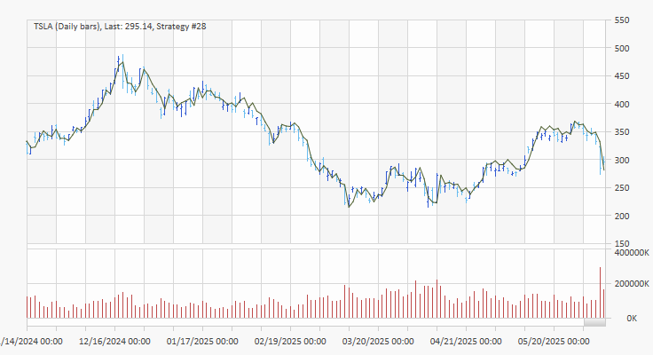
Figure 3. Predicted prices of TSLA superimposed on the price chart. The prices are determined from the predicted price changes. The data shown are for the validation (out-of-sample or OOS) segment.
Some of the build results are shown below for the training and validation (OOS) segments. Notice that the results on the OOS segment are better for almost all metrics than on the training segment, a pattern that repeated across all the examples. For the Net Points and Net Points/Bar metrics, this is due in part to the increasing price of TSLA over time, which increases by approximately 200x from the beginning of the training data to the end of the validation segment.
| Metric | Training | OOS |
|---|---|---|
| MSE | 0.0378 | 0.0341 |
| Net Points | 184 | 370 |
| Net Points/Bar | 0.061 | 1.313 |
| Dir Correct (Pct) | 50.9% | 54.6% |
| Ave Error (Pct) | 3.20% | 3.72% |
Finally, I retrained the network using the Adam method to compare the training processes and results. Because the weights are initialized randomly, different results are generally obtained from each training run. In most cases, the results from Adam were quite close to the results shown above. The convergence of the Adam training method is depicted below in Fig. 4. Each "epoch" represents the results from applying the Adam method based on the gradient calculated from the samples in one batch (32 samples). In general, the training process using Adam converged much faster than using the genetic optimizer.
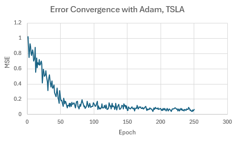
Figure 4. Mean squared error (MSE) versus epoch for TSLA trained via Adam.
BTC-USD. For bitcoin, I used the same build settings as shown in Fig. 1 except that due to the larger size of bitcoin relative to TSLA, I increased the condition for net points per bar to 25 based on a preliminary build. The build process resulted in the following inputs:
                            Input 1:  TrueRange[19]
                            Input 2:  AS_PivotR(3)
                            Input 3:  Momentum(H, 55)
AS_PivotR is the pivot resistance price, which is one of the built-in indicators of Adaptrade Builder.
The predicted prices, inferred from the predicted price changes, are shown below in Fig. 5 for the top strategy on the validation (OOS) segment.
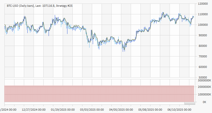
Figure 5. Predicted prices of BTC-USD superimposed on the price chart. The prices are determined from the predicted price changes. The data shown are for the validation (OOS) segment. Note: The volume graph is incorrect due to the size of the values, which exceed the available display limit.
Some results are shown below for the training and validation (OOS) segments. As with TSLA, the results not only hold up well in the OOS segment but are better in some cases than on the training segment.
| Metric | Training | OOS |
|---|---|---|
| MSE | 0.0528 | 0.0534 |
| Net Points | 119929.3 | 57141.4 |
| Net Points/Bar | 38 | 169 |
| Dir Correct (Pct) | 51.8% | 53.9% |
| Ave Error (Pct) | 4.49% | 2.87% |
The results to this point have been for predicting the price change for the next bar. To see how well the LSTM could predict the price change at longer prediction lengths, I tried prediction lengths from 1 to 50 bars, keeping everything else the same. The results are shown below in Fig. 6, where it can be seen that much higher prediction accuracies are achieved at longer prediction lengths.

Figure 6. Effect of prediction length on direction accuracy for BTC-USD. The data shown are for the validation (OOS) segment.
At first, this may seem counter-intuitive since most prediction methods tend to lose accuracy when the prediction window is extended, such as with weather forecasting. However, financial market prices contain a large component of noise, which means that the direction of price change for the next bar in a price series is probably mostly random. This is supported by the results in Fig. 6 for the first few data points where the prediction accuracies are not much better than 50%. As the prediction length increases, the accuracy starts to steadily increase as well. This is consistent with the idea that at longer prediction lengths, the signal-to-noise ratio should be much larger.
QQQ. I used the same build settings for the Nasdaq 100 ETF (QQQ) as for TSLA (see Fig. 1). The build process resulted in the following single input:
Input: Momentum(TypicalPrice[4], 30)
For comparison to the other examples, the following table lists some results for the training and validation segments:
| Metric | Training | OOS |
|---|---|---|
| MSE | 0.0427 | 0.0461 |
| Net Points | 67.1 | 291.4 |
| Net Points/Bar | 0.0127 | 0.469 |
| Dir Correct (Pct) | 51.2% | 53.5% |
| Ave Error (Pct) | 1.49% | 1.17% |
One question I have not yet addressed is the effect of the size of the neural network on the results. Each of the preceding examples used the same size network: 100 nodes per layer or approximately 200,000 weights (depending on the number of inputs). To explore the effect of network size on the results, I increased the number of nodes per layer from 25 to 250 for the input shown above (and keeping all other settings the same) and recorded the mean squared error for each network after retraining it via the Adam method. The results are shown below in Fig. 7.

Figure 7. Effect of neural network size (number of nodes per layer) on the MSE for QQQ with one input and three hidden layers.
Beyond 100 nodes per layer, it can be seen that the MSE does not change much for either the training or OOS segments. For reference, the relationship between the number of nodes per layer and the total number of weights in the neural network for this specific LSTM network (1 input, 1 output, 3 hidden layers) is shown in Fig. 8. As shown in the figure, with 250 nodes per layer, the LSTM had about 1.2 million weights. It should be noted that the relationship between the MSE and the number of nodes per layer is probably dependent on the amount of input data. For the daily QQQ data used here, there were about 5300 bars in the training segment. If much more data was used, it's likely that larger networks would be more effective than shown here.
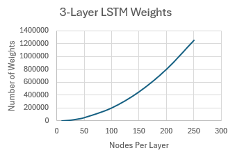
Figure 8. Relationship between total number of weights and number of nodes per layer for an LSTM with 1 input, 1 output, and 3 hidden layers.
ES. As shown in Fig. 6 for the bitcoin example, much better prediction accuracies are seen when the prediction length is increased. The prior examples were all based on daily bars, for which a longer prediction length would preclude short-term trading strategies. This raises the question: if you want to use an LSTM for short-term trading, will it also work on intraday data? To answer that question, I trained an LSTM network on 15-minute bars of the E-mini S&P 500 futures (symbol ES).
Most of the settings were the same as shown in Fig. 1, except for the following. I set the prediction length to 30 bars, the initial number of inputs to 3, the condition for the percent of correct direction predictions to 60%, and the condition for the net points per bar to 0.2. The build process resulted in the following input:
Input: Momentum(L[17], 81)
The results for the training and validation segments are shown below.
| Metric | Training | OOS |
|---|---|---|
| MSE | 0.0757 | 0.0752 |
| Net Points | 29308 | 4221 |
| Net Points/Bar | 0.230 | 0.265 |
| Dir Correct (Pct) | 60.4% | 60.8% |
| Ave Error (Pct) | 0.45% | 0.31% |
As with the other examples, the results on the OOS segment are similar to and, in some cases, slightly better than those on the training segment. For the prediction length of 30 bars, the directional accuracy was about 60% on both segments, suggesting that the LSTM neural network has potential on intraday data, similar to the results on daily bars. It's also interesting to notice that the accuracy of 60% for a prediction length of 30 bars is very similar to the prediction accuracy on daily data for BTC-USD at this length, as shown in Fig. 6.
Summary and Discussion
There are several takeaways from this work and, at least for me, two surprises. First, it seems that deep neural networks, and, in particular, the LSTM architecture are fairly effective in predicting market price changes. In each of the examples, which spanned four different instruments — a stock, a cryptocurrency, an ETF, and an index future — positive results were obtained: the Net Points metric was positive in each case. I should note that this may not have been the case had I trained these networks using just the MSE. Including metrics such as Net Points/Bar probably helped achieve results that have more potential for trading.
Another observation worth reiterating is that the prediction for the next bar was not much better than random. While the metrics related to potential trading profits (Net Points and Net Points/Bar) were still positive, the directional accuracy in predicting the next bar was not much higher than 50%. This is most likely due to the large amount of noise in market prices. For example, when viewing a price chart, the trends that develop over many bars tend to stand out whereas the directional change of any particular bar can appear to be random.
This leads to the first surprise; namely, that the prediction accuracy is much higher for longer prediction lengths. While perhaps obvious in hindsight, especially considering the observation noted in the preceding paragraph, it's a much different result than would normally be expected from a prediction model. However, models based on physics, such as for weather prediction, work much differently than neural networks. In a physics-based model, the simulation starts from a set of initial conditions and works forward, time step by time step, where each time step builds on the last one. As a result, errors compound and accuracy decreases over successive steps.
A neural network, on the other hand, looks for patterns. If those patterns are more obvious, such as with multi-bar trends, as opposed to the direction of the next bar, it makes sense that the neural network would be better able to identify the pattern. Put another way, longer-term patterns have a higher ratio of signal (the non-random part) to noise (the random part), which makes the pattern easier to "see".
The second surprise was how well the results held up in the OOS segment. Arguably, one of the biggest obstacles that systematic traders face is trading strategies that fail to generalize beyond the training or optimization data. Whether it's a result of overfitting or changes in market dynamics, many technical and systematic trading approaches look great in hindsight (i.e., during development or optimization) but fail in real time or when applied to data not used in their development.
In all the examples I've studied so far with these LSTM networks, including the examples shown here, the OOS results have been very close in performance to the results on the training segment without the benefit of any selection bias. This is also somewhat surprising from a statistical point of view because the number of parameters (weights) in the model is vastly greater than the number of input data used to train the model. However, this is common with deep neural networks, which often generalize well despite being overparameterized. Overfitting can still be a concern, though the batch training approach used here helps introduce randomness into the training process. It's also conceivable that the noise component in market prices provides a built-in regularization effect in that the prices themselves have a large component of randomness.
This article introduced the LSTM feature I've been developing for Adaptrade Builder, but more work remains to be done. In the next article, I'll show how the LSTM networks can be incorporated into trading strategies. The main challenges will be (1) effectively using the neural network predictions in combination with other strategy logic and (2) implementing the neural network inference process given the relatively large size and complexity of the LSTM networks and the limitations of conventional scripting languages for trading.
References
- Krizhevsky, A., Sutskever, I., Hinton, G. ImageNet Classification with Deep Convolutional Neural Networks, NIPS, 2012.
- Goodfellow, I., Bengio, Y., Courville, A. Deep Learning, The MIT Press, Cambridge, MA, 2016, pp. 397-400.
- Hochreiter, S., Schmidhuber, J. Long short-term memory, Neural Computation, 9 (8), 1997, pp. 1735-1780.
- Dixon, M., Klabjan, D., and Bang, J. H. Classification-based Financial Markets Prediction using Deep Neural Networks, 2016. https://arxiv.org/abs/1603.08604
- Kelly, B., Xiu, D. Financial Machine Learning, 2023, pp. 67-70. https://ssrn.com/abstract=4501707
- Fischer, T., Krauss, C. Deep learning with long short-term memory networks for financial market predictions, European Journal of Operational Research, 270 (2), 2018, pp. 654-669.
- Goodfellow, I., Bengio, Y., Courville, A. Deep Learning, The MIT Press, Cambridge, MA, 2016, pp. 301-302.
Good luck with your trading.
Mike Bryant
Adaptrade Software
This article appeared in the July 2025 issue of the Adaptrade Software newsletter.
HYPOTHETICAL OR SIMULATED PERFORMANCE RESULTS HAVE CERTAIN INHERENT LIMITATIONS. UNLIKE AN ACTUAL PERFORMANCE RECORD, SIMULATED RESULTS DO NOT REPRESENT ACTUAL TRADING. ALSO, SINCE THE TRADES HAVE NOT ACTUALLY BEEN EXECUTED, THE RESULTS MAY HAVE UNDER- OR OVER-COMPENSATED FOR THE IMPACT, IF ANY, OF CERTAIN MARKET FACTORS, SUCH AS LACK OF LIQUIDITY. SIMULATED TRADING PROGRAMS IN GENERAL ARE ALSO SUBJECT TO THE FACT THAT THEY ARE DESIGNED WITH THE BENEFIT OF HINDSIGHT. NO REPRESENTATION IS BEING MADE THAT ANY ACCOUNT WILL OR IS LIKELY TO ACHIEVE PROFITS OR LOSSES SIMILAR TO THOSE SHOWN.