
Adaptrade Software Newsletter Article
Portfolio Composition and Optimization
It's well established that one of the best ways to increase risk-adjusted returns is diversification. That's why most professional traders trade a portfolio of market systems, rather than just one market or one strategy. However, putting together a good portfolio can be more complicated than just combining your best market systems. For example, the performance of the portfolio will depend on how you allocate capital to each market system. And what if you have more market systems than you can reasonably trade? How do you select the best subset of available market systems to trade?
This article will address these questions. In particular, I'll start by presenting the equation for the number of combinations of market systems in a portfolio. The equation makes it clear that it's not practical to consider every possible combination except for small portfolios. I'll then present several objective methods for identifying candidate market systems to remove from a portfolio in order to reduce its size. I'll also demonstrate the process of optimizing the position sizing for a portfolio, which determines the allocations to the market systems. Lastly, I'll present out-of-sample tests to validate the portfolio composition decision and to estimate the bias from the position sizing optimization.
Combinations of Market Systems
Diversification is one of the only true "free lunches" in trading and investing. However, a large number of market systems can become too much of a good thing. While dozens of stock symbols might be manageable in a buy-and-hold investment portfolio, for trading, particularly for short-term trading, managing a large number of market systems is much more difficult. If you're an individual trader without a supporting team to help manage your trades, you might feel you can successfully manage only a handful of markets at the same time. Also, if two market systems are highly correlated, there could be little benefit to trading both unless, perhaps, they trade different markets and your position sizes are so high that you need the liquidity of both markets.
To be clear, what really matters is how the market systems trade with respect to each other, not necessarily whether the underlying symbols are correlated. For example, you could have a short-term strategy on the E-mini S&P futures and a long-term, trend-following strategy on the same symbol. Even though both strategies trade the same symbol, the market systems (i.e., the combination of the symbol and the trading strategy) could have a very low correlation to each other. On the other hand, you might be trading two different strategies with similar underlying logic on two different but correlated symbols. Even though the strategies and markets are different, the market systems might be highly correlated.
So, what do you do if you have more market systems than you can reasonably trade? Ideally, you'd like to be able to test every possible combination of market systems, optimize each combination, and choose the best one. For example, let's say you have five market systems that you want to trade but you only have the capital to trade two of them. If the market systems are numbered 1 to 5, then there are 10 possible combinations of two market systems: (1, 2), (1, 3), (1, 4), (1, 5), (2, 3), (2, 4), (2, 5), (3, 4), (3, 5), and (4, 5).
In general, the number of combinations of n market systems taken m at a time can be expressed in terms of the binomial coefficient1 as follows:
C(n, m) = n!/[m! (n - m)!]
where "!" represents the so-called factorial function; i.e., x! = x * (x - 1) * (x - 2) * (x - 3) * ... * 2 * 1.
The total number of combinations of n market systems is therefore simply the sum of C(n, m) over all values of m:
C(n) = Σm=1..nC(n, m).
This equation adds up the numbers of combinations of n market systems taken m at a time for all values of m; i.e., the number of combinations of one market system plus the number of combinations of two market systems plus the number of combinations of three market systems and so on.
For small values of n, the total number of combinations, C(n), is reasonably small. For example, for 10 market systems, C(10) = 1023. If you could automate the process of evaluating and optimizing all 1023 combinations, it might be reasonable to do so. However, for 20 market systems, C(20) = 1048575. Evaluating and optimizing more than one million combinations is probably not practical. If trying every possible combination of market systems is not feasible, then what approach is more reasonable for solving the portfolio composition problem?
Methods to Reduce the Size of a Portfolio
If we have a portfolio that is larger than we can trade, an obvious solution is to start with all possible market systems then remove one or more market systems until the portfolio is small enough. If we have a method for removing a single market system from the portfolio, we can apply it repeatedly until the portfolio is small enough. With that in mind, the following three methods for removing a market system from a portfolio in order to reduce its size will be considered:
- Remove the market system with the worst individual performance, such as the lowest net profit, smallest profit factor, or lowest Sharpe ratio.
- Optimize the portfolio and remove the market system with the lowest position sizing parameter. In this context, optimization refers only to the position sizing for the market systems, not the rules or parameters of the trading strategies, which are assumed to be fixed.
- Add up the correlation coefficients of each market with respect to every other market system. Remove the market system with the highest total correlation.
The first method is intuitively obvious. The market system to remove can be identified by examining the individual results on a fixed contract (share) basis or by analyzing the full portfolio on an equal-weight basis and examining each market system's contribution to the overall portfolio results.
The second method requires that the full portfolio is optimized first. Optimization should help identify the weakest market system. That's because optimizing the position sizing for the portfolio will tend to allocate more equity to the better market systems and less to the worse ones. For example, if you use fixed fractional position sizing for each market system in the full portfolio, the weakest market system will be the one with the smallest fixed fraction after optimization.
The third method is based on the idea that if two market systems are highly correlated, you probably don't need both. However, each market system has correlations with every other market system, so rather than looking at a single correlation coefficient between two market systems, we'll add up all the correlation coefficients of each market system with every other one. In practice, this means adding up each row in the table of correlation coefficients and removing the market system corresponding to the row with the highest total. Since optimizing the portfolio will affect the correlation coefficients, this method will be based on the correlation coefficients of an equal-weight portfolio.
Admittedly, each of these methods is ad hoc. They are not guaranteed to produce the optimal portfolio of the next lowest size. To do that, it would be necessary to remove each market system in turn from the portfolio, optimize the reduced portfolio, and compare the different optimized portfolios to find which removed market gives the best result. For a portfolio of n market systems, this would require n optimizations to remove the first market system. To remove the next market system would require n - 1 optimizations, and so on. While the three methods above are not definitive, in practice, they will likely give the same result as systematically removing each market system in turn and will only require, at most, three optimizations to generate the results needed to compare the different methods.
A Stock Trading Example
To illustrate the process of selecting a market system to remove from a portfolio, a trading strategy was built on 30-minute bars of the following stocks: Apple (AAPL), Amazon (AMZN), Facebook (FB), Google (GOOG), Netflix (NFLX), and Tesla (TSLA). The strategy was built using Adaptrade Builder over the date range July 15, 2015 to May 23, 2019. The purpose of the strategy was only to provide a set of trades for a hypothetical portfolio; the details of the strategy are not relevant to this article. The list of trades generated by the strategy over the six markets was saved from Builder to a set of files for Market System Analyzer (MSA). These files included a market-system file for each market plus a portfolio file for the combination of all six market systems.
Because the portfolio composition and optimization decisions benefit from hindsight, the data were divided into in-sample and out-of-sample periods: 7/24/15 - 5/23/18 (in-sample) and 5/24/18 - 5/23/19 (out-of-sample). All decisions were made based on the in-sample results. As shown later, the results on the out-of-sample period were used to evaluate the composition and optimization decisions. The equity curves, as plotted in MSA, are shown in Fig. 1 for the in-sample period.
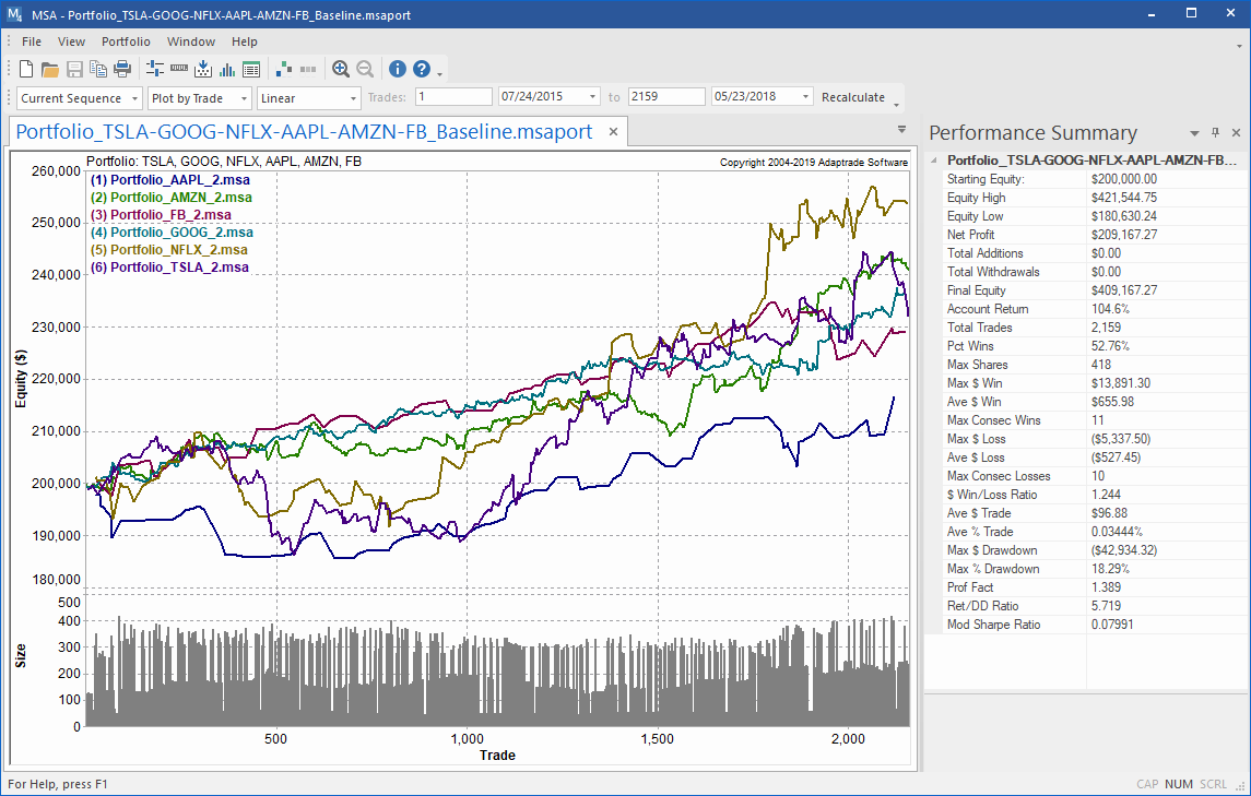
Figure 1. Equity curves for each market system in a stock trading portfolio example. Positions are based on an equal weighting of 16.67% of equity per trade.
The results depicted in Fig. 1 represent the baseline portfolio with equal-weight position sizing. In MSA, this means the position sizing for each market system was set to "percent of equity" with a percentage value of 16.67% (i.e., 100% divided by six). This position sizing method sets the size for each trade so that the value of the position is the specified percentage (16.67% in this case) of account equity.
Method 1: Worst Performer
The worst performing market system of the baseline portfolio can be identified from the results broken out by
market system, as shown below in Fig. 2. The market system for AAPL has the lowest net profit and Sharpe ratio and the
second-smallest profit factor.
For those reasons, the AAPL market system is arguably the worst performing one in the portfolio, suggesting it should be removed.
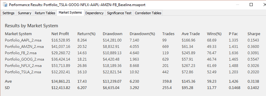
Figure 2. Results by market system for the baseline (equal weight) portfolio.
Method 2: Weakest After Optimization
To evaluate the weakest market in the optimized portfolio, position sizing optimization was performed on the baseline portfolio.
The genetic optimizer of MSA was used to find the optimal parameter values for percent-of-equity position sizing for each
market system. The optimization was performed twice. First, the process was started at random values chosen by the program. In the
second pass, the optimization was started at the optimal values found during the first pass. The optimization settings and results
are shown below in Fig. 3. Note that for portfolio optimization, the position sizing parameter (e.g., percent of equity) is applied
to the portfolio equity. As can be seen in the figure, the market system for AAPL has the lowest position sizing parameter
value (0.03%), suggesting it should be removed.
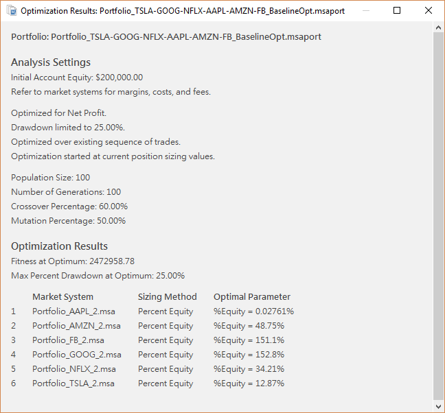
Figure 3. Optimization of the baseline portfolio.
Method 3: Total Correlation Coefficient
To calculate the sum of the correlation coefficients of each market system with respect to the others, the correlation
tables calculate by MSA were copied to Excel, and the rows were summed. MSA calculates a table of correlation coefficients for
different time periods (daily, monthly, annual), as well as based on the detrended equity curves. The sums of the coefficients were
calculated for each table, as shown below in Fig. 4, where the totals are listed in the right-hand column, with the highest total
for each table highlighted in red. In this case, the highest total for each table is for market system #5,
suggesting that the market system corresponding to NFLX should be removed. If different correlation tables had identified different
market systems, you could either make a judgement about which result was more meaningful or try removing each identified market
system in turn.
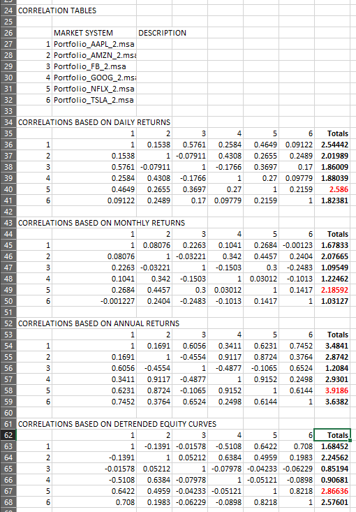
Figure 4. Correlation coefficients of the baseline portfolio.
In summary, among the three methods, two market systems were identified as candidates for removal from the portfolio: AAPL (via methods 1 and 2) and NFLX (via method 3). The next step is to remove each market system one at a time and optimize the reduced portfolio. The optimal results will then be compared to identify the best portfolio, and, finally, the out-of-sample results will be evaluated.
Optimal Reduced Portfolios
Each reduced portfolio was optimized by first removing the identified market system — by unchecking either AAPL or NFLX
in the "Include" column of the Portfolio Setup window of MSA — then
applying the same optimization process as described above (Fig. 3) in which the net profit was maximized subject to a limit on the
maximum drawdown of 25%. Given the optimization objectives, the optimal reduced portfolios will be compared based on the
resulting net profit, assuming the drawdown constraint was met in each case. The portfolio with the greatest net profit at a maximum
drawdown level of 25% will be deemed the best portfolio.
The results are shown below in Table 1. For comparison, the baseline portfolio is included in the table. As shown in the table, the best portfolio is the one in which the market system for AAPL has been removed. The corresponding reduced portfolio has 83% more net profit over the in-sample period than the baseline portfolio for the same maximum drawdown. The portfolio with the market system for NFLX removed actually performed worse than the baseline portfolio.
| Removed | Net Profit | Max Drawdown (%) |
|---|---|---|
| NA (Baseline) | $2,473,277 | 25.0 |
| AAPL | $4,532,776 | 25.0 |
| NFLX | $2,282,280 | 25.0 |
The equity curves for the optimized portfolio with the market system for AAPL removed are shown below in Fig. 5. Notice that the lowest equity curve on the plot, which corresponds to FB, shows a net loss. However, if this market system is removed from the portfolio (without re-optimizing), the portfolio net profit drops and the worst-case drawdown increases. This is because the market system for FB is negatively correlated with most of the other market systems, so it tends to produce profits when the other market systems are losing and vice-versa. Even though its net profit is negative overall, when it's profitable, those profits allow the other market systems to trade more, which more than offsets the losses from FB.
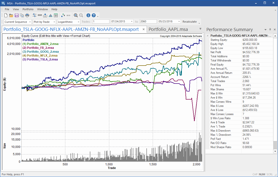
Figure 5. Equity curves for each market system in the portfolio with the market system for AAPL removed. The reduced portfolio was optimized for "percent of equity" position sizing.
Out-of-Sample Results
Two different tasks were performed above: composition and optimization. Both should be tested out-of-sample. The composition task was removing the market system for AAPL from the portfolio. We want to know if this decision holds up out-of-sample. The optimization task was optimizing the portfolio after removing the market system for AAPL. For this task, we want to know how much bias was introduced by the optimization.
To test the composition task out-of-sample, we can compare the out-of-sample results for the optimized baseline portfolio (i.e., including the market system for AAPL) to the out-of-sample results for the optimized portfolio without the market system for AAPL. As shown above in Table 1, the in-sample results excluding the market system for AAPL are much better than for the baseline portfolio. We want to confirm that the same is true out-of-sample. The out-of-sample comparison is shown below in Table 2.
| Portfolio | Net Profit | Max Drawdown (%) |
|---|---|---|
| Baseline | $306,520 | 36.7 |
| Reduced (AAPL) | $577,531 | 27.4 |
The results in Table 2 confirm that the reduced portfolio is also better out-of-sample. The net profit is greater and the worst-case drawdown is lower than that of the baseline portfolio on the out-of-sample period.
To estimate how much bias was introduced by optimizing the reduced portfolio, we can move the optimization window forward so that the new in-sample period includes the former out-of-sample period. We can then compare the new optimized results to the out-of-sample results from the prior optimization over the same time period (i.e., 5/24/2018 - 5/23/2019). In this way, we'll be comparing in-sample results to out-of-sample results over the same time period. The difference will tell us how much bias is introduced by the optimization.
The new optimization window is 7/24/2016 to 5/23/2019. The reduced portfolio was optimized over this range using the same procedure as above. Following the optimization, the date range was restricted to the original out-of-sample period (5/24/2018 - 5/23/2019), and the results were recalculated. Table 3 shows how these new, optimized results compare to the prior out-of-sample results over the original out-of-sample period.
| Portfolio | Net Profit | Max Drawdown (%) |
|---|---|---|
| Optimized | $916,732 | 26.2 |
| Out-of-Sample | $577,531 | 27.4 |
As expected, including the trades from the original out-of-sample period in the optimization yields better results over that period as compared to the out-of-sample results, which come from optimizing without the benefit of those trades. The ratio of the out-of-sample to optimized net profit over the original out-of-sample period is 577531/916732 = 0.63. So, we might expect that our net profit will about 63% as much as the optimization results suggest. Of course, this is only one out-of-sample comparison. Doing repeated walk-forward optimizations would give other data points. Notably, the drawdown is about the same out-of-sample as from the optimized results.
Discussion
Putting together a good portfolio of market systems requires two basic tasks: deciding which market systems to include in the portfolio and optimizing the allocations to the market systems (i.e., position sizing). Both tasks were examined above. As the example illustrated, the composition task is related to the optimization task. Ultimately, the only way to know if the portfolio composition is optimal is to optimize the portfolio and compare it to other optimized portfolios of different compositions.
Because portfolio position sizing optimization itself can be a time-consuming process, an approach was presented to limit the number of different portfolios that need to be optimized. Rather than optimizing every possible combination of n market systems taken m at a time (i.e., C(n, m) combinations), three objective methods for removing a market system from a portfolio were presented. To reduce the size of a portfolio from n to m, the three methods need to be repeated n - m times. This means it will take 3 * (n - m) optimizations to reduce a portfolio to m market systems. Since C(n, m) is factorial in n, 3 * (n - m) will be smaller than C(n, m) for almost all values of n and m. For example, for n = 10 and m = 8, C(10, 8) = 45, whereas 3 * (10 - 8) = 6.
A potential problem with any type of optimization is over-fitting. To assess that risk, out-of-sample testing was performed on both the portfolio composition and the optimization results. Different out-of-sample tests were used for each decision. To test the composition decision out-of-sample, the reduced portfolio was compared to the baseline portfolio in the out-of-sample period. Notice that this test is not as strict as comparing the reduced portfolio in the out-of-sample period to the optimal portfolio found by applying the composition process to the out-of-sample trades. Nonetheless, it demonstrated that the composition decision held up through the out-of-sample period.
To test the position sizing optimization out-of-sample, a test was devised to estimate the bias introduced by the optimization process. This test is similar to the walk-forward testing approach developed by Pardo2 in which the out-of-sample results of repeated walk-forward tests are evaluated relative to the in-sample results to estimate the so-called "walk-forward efficiency". The difference here is that the out-of-sample results are compared to the optimized results over the same time period. In this case, the test was used to estimate, albeit roughly, the expected results as a percentage of the optimized (in-sample) results.
The portfolio optimization considered in this article was for position sizing only. It was assumed that the strategy logic and associated parameter values for each trading strategy were fixed. This has the advantage of separating strategy design from portfolio composition and position sizing, thereby simplifying each. However, it's likely that a strategy's logic will influence how it combines with other market systems, affecting the portfolio composition. (To some extent, this was implicitly taken into account during the strategy building process by Adaptrade Builder because it was directed to build a strategy that worked well over all six markets as a portfolio.) Strategy logic can be also be combined with position sizing, such as by increasing the position size if certain favorable market conditions are met. While it's true that all of these factors potentially interact with each other, trying to simultaneously optimize strategy logic, position sizing, and portfolio composition would be a formidable problem.
Portfolio composition and optimization should be as fundamental to traders as they are to investors. Hopefully, the topics discussed in this article will provide some food for thought for your future portfolio trading plans.
References
- https://en.wikipedia.org/wiki/Binomial_coefficient.
- Pardo, R. Design, Testing, and Optimization of Trading Systems, John Wiley & Sons, Inc., New York, 1992.
Good luck with your trading.
Mike Bryant
Adaptrade Software
This article appeared in the June 2019 issue of the Adaptrade Software newsletter.
HYPOTHETICAL OR SIMULATED PERFORMANCE RESULTS HAVE CERTAIN INHERENT LIMITATIONS. UNLIKE AN ACTUAL PERFORMANCE RECORD, SIMULATED RESULTS DO NOT REPRESENT ACTUAL TRADING. ALSO, SINCE THE TRADES HAVE NOT ACTUALLY BEEN EXECUTED, THE RESULTS MAY HAVE UNDER- OR OVER-COMPENSATED FOR THE IMPACT, IF ANY, OF CERTAIN MARKET FACTORS, SUCH AS LACK OF LIQUIDITY. SIMULATED TRADING PROGRAMS IN GENERAL ARE ALSO SUBJECT TO THE FACT THAT THEY ARE DESIGNED WITH THE BENEFIT OF HINDSIGHT. NO REPRESENTATION IS BEING MADE THAT ANY ACCOUNT WILL OR IS LIKELY TO ACHIEVE PROFITS OR LOSSES SIMILAR TO THOSE SHOWN.