Detecting Nonrandomness in the Markets
Economists
have long debated whether stock market prices change randomly or are at
least partially predictable.
The random walk hypothesis says that stock market prices change in a
random fashion, making prediction impossible. However, more recent
research has uncovered a variety of inefficiencies in the markets that
disprove the random walk hypothesis. Certainly, any trader who has
followed the markets for any length of time, let alone successfully
traded them, doesn't need an academic study to tell them the markets are
not entirely random. Nonetheless, there's some benefit to being able to
demonstrate it mathematically.
The autocorrelation is a
statistical measure that is often used to detect nonrandomness in noisy
data. For example, if a sine wave is hidden in a noisy electromagnetic
signal, the autocorrelation might be used to detect it. The
autocorrelation measures the degree of correspondence between a signal
and an offset version of the signal. Technically, the autocorrelation is
the correlation coefficient of a signal and the signal delayed by a time
increment called the lag. The correlation coefficient, and therefore the
autocorrelation, returns a value in the range -1 to +1. Values close to
either -1 or +1 indicate a high degree of nonrandomness. Values close to
zero indicate randomness.
When applying the
autocorrelation to market prices, we want to analyze the price changes,
rather than the price itself. Price changes often appear to be random. If the price
changes have any serial correlation, it will show up in the
autocorrelation. In this case, the lag is the number of bars the series
of price changes is offset when comparing it to the original series.
For example, consider the
following series of price changes:
0, -4, 0.5, 0.5, 3.25, 9.75,
4.5, 21.25, 3.5, -2, -9, 3, -3, -15.5, 0.25, -21, 2.75, 20.25, 0.5
These were obtained by
subtracting the prior close from the current close for a short segment
of daily bars in the E-mini S&P 500 futures. The autocorrelation at lag
1 for these data would be the correlation coefficient of the following
two series:
-4, 0.5, 0.5, 3.25, 9.75, 4.5,
21.25, 3.5, -2, -9, 3, -3, -15.5, 0.25, -21, 2.75, 20.25, 0.5
and
0, -4, 0.5, 0.5, 3.25, 9.75,
4.5, 21.25, 3.5, -2, -9, 3, -3, -15.5, 0.25, -21, 2.75, 20.25
Notice that the second series
is just the first one offset by one bar.
The correlation coefficient is
defined as the covariance divided by the variance. TradeStation's
EasyLanguage contains functions for calculating both the covariance and
variance of arrays, so these can be used to calculate the
autocorrelation. For example,
Value1 = CovarArray(DeltaP,
DeltaPLag, NBars);
Value2 = VarianceArray(DeltaP, NBars, 1);
AutoCorr = 0;
If Value2 > 0 then
AutoCorr = Value1/Value2;
Above, DeltaP is the array of
price changes over the past NBars bars, and DeltaPLag is the array of
price changes starting Lag bars back. The complete indicator code is
available online on the
download page.
In addition to calculating the
autocorrelation value itself, it's also necessary to determine the level
at which the value is statistically significant. There are several
references available online that provide the appropriate formula, such
as
http://en.wikipedia.org/wiki/Correlogram and
http://www.ltrr.arizona.edu/~dmeko/notes_3.pdf. An approximate
formula for the 95% confidence bands is:
±
2/sqrt(NBars)
where "sqrt" is the square root
operator. For example, for NBars equal to 100, the confidence bands are
+0.2 and -0.2. That means any value of autocorrelation greater than or
equal to 0.2 or less than or equal to -0.2 is considered statistically
significant.
I created two versions of the
autocorrelation indicator for TradeStation. Both versions plot a line
for the autocorrelation value and lines for the confidence limits. Any
value outside the confidence limits is colored differently to highlight
the fact that it's statistically significant. The first indicator,
simply called "Autocorrelation" calculates the autocorrelation of
closing price changes over the past NBars bars at lag Lag, where NBars
and Lag are inputs. For example, you could use it to plot the
autocorrelation over the past 30 bars with a lag of 2.
The other version, named
AutocorrMax, is designed to detect significant autocorrelation values
for a range of lags from 1 to the input value MaxLag. For example, if
MaxLag is 20, the indicator will calculate the autocorrelation for lags
1, 2, 3, ..., 20. The largest autocorrelation (absolute) value is
recorded and plotted.
Nonrandomness in the E-mini
S&P
To illustrate the use of the
autocorrelation indicators, I applied them to daily bars of the E-mini
S&P 500 futures from 5/17/2006 to 11/19/2010. The application of
AutocorrMax is more interesting in that it finds areas where the
autocorrelation is significant for any of the lag values from 1 to
MaxLag. As a result, there are more statistically significant values
than from looking only at a specific lag. I applied this indicator with
a MaxLag value of 20 and NBars equal to 100. This means it calculated
the autocorrelations over the prior 100 bars for lags from 1 to 20.
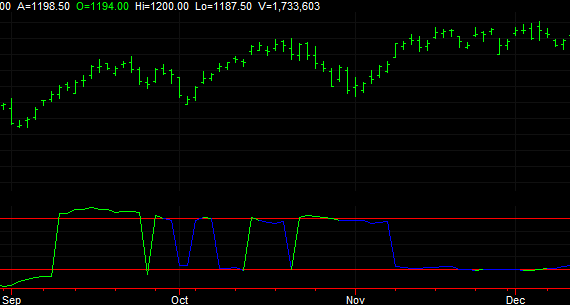
Figure 1. Maximum
autocorrelation values over the past 100 bars for lags 1 to 20. Green
indicates statistical significance.
A sample of the E-mini S&P
chart is shown in Fig 1. When the maximum autocorrelation value over the
different lags is statistically significant (i.e., above the upper band
or below the lower band), the indicator plots the value in green. Where
the green line crosses from one band to the other, as shown above, the
maximum autocorrelation changes from positive to negative from one bar
to the next.
Significantly positive values
of autocorrelation indicate that the price changes are positively
correlated. In other words, a positive price change tends to lead to
another positive price change over the lag period. Significantly
negative autocorrelations tended to be more prevalent in the chart. A
typical period of statistically significant negative correlation is
shown below in Fig. 2.
Figure 2. Maximum
autocorrelation values over the past 100 bars for lags 1 to 20. Green
indicates statistical significance.
As shown above, the maximum
autocorrelation stays significantly negative for several months.
Negative autocorrelation means that the price changes tend to reverse.
For example, a positive price change tends to precede a negative price
change, and vice-versa.
To estimate how much of the
E-mini S&P's price behavior is nonrandom, I saved the indicator values
to a file. I opened the file in Excel and tabulated all values that were
statistically significant. I found that 62% of price bars in the file
had a significant level of autocorrelation, either positive or negative.
By this measure, then, 38% of the price changes are random and 62% are
nonrandom. It's likely, however, that repeating the calculation with
different look-back lengths (NBars) would yield different results.
Keep in mind that the
AutocorrMax indicator, as shown in the figures, doesn't show us which
lag was statistically significant. It may be that the autocorrelation
was significant for several lags or just one. If you want to know which
lag was responsible for the significance, you can plot the
Autocorrelation indicator for individual lags to test which ones are
significant.
Although I didn't test this,
the autocorrelation indicators could potentially be used as trading
filters. For example, you might try restricting trend trades to periods
where the maximum autocorrelation over a range of lags, as in the
AutocorrMax indicator, is significantly positive. Likewise, a
counter-trend system might benefit by filtering entries to periods where
the autocorrelation is negative.
Conclusions
The autocorrelation calculation
lends support to one of the foundations of technical trading; namely,
that the markets contain nonrandom price behavior that can be exploited.
Calculating the autocorrelation for a range of lags allows us to uncover
a wider range of nonrandomness than focusing on a single lag.
Applying the autocorrelation
indicator to the E-mini S&P revealed more periods of negative
correlation than positive correlation. It also suggested that there are
extended periods of significant autocorrelation and that, overall, the
E-mini S&P has a substantial amount of nonrandomness.