The following article was originally published in the September 2011 issue of The Breakout Bulletin.
 

Intermarket Correlations in the E-mini

When the markets are trading and I'm not in front of the computer, I sometimes tune in to CNBC for a quick update. I'll glance at the S&P, Dow, NASDAQ, 10 year T-notes, gold, crude oil, and maybe another market or two. In only a few moments, I feel like I know what's going on. I've just done a quick and intuitive form of intermarket analysis.

Generally speaking, intermarket analysis means looking at how other markets relate to and influence the market you're trading. In developing a trading strategy, it might be reasonable to think that intermarket analysis would be useful when two markets are correlated, whether the correlation is positive (i.e., the markets tend to move together) or negative (i.e., the markets tend to move in opposite directions). But how can you know if that's the case?

In order to test that idea, it's first necessary to decide how to incorporate the correlations between markets into a trading strategy. The problem is that there are many different ways that correlations might be used in a trading strategy. For example, the correlation between two markets can be compared to a threshold value; the correlations between pairs of markets might be tested to see which markets contribute to the strategy; correlations between different markets might be compared to each other; and so on. Testing every possible idea is probably not feasible.

Fortunately, genetic programming can be used to solve this problem. In genetic programming (GP), the algorithm constructs a trading strategy using selected elements of strategy logic, such as the correlations between markets. The GP algorithm combines the logical elements in a way that both makes sense and provides the best strategy results. In this way, it's not necessary to specify beforehand how the correlations are to be used; the GP algorithm determines that.

For this problem, I chose the E-mini S&P 500 (ES) futures as the trading vehicle, as shown below in Fig. 1. I wanted to see which other markets, if any, were useful in trading the ES. I chose the following candidate markets:

E-mini NASDAQ 100 futures (NQ)

E-mini Euro FX futures (E7)

E-mini Crude Oil (QM)

Dow Jones CBOT Treasury Index (DJCBTI)

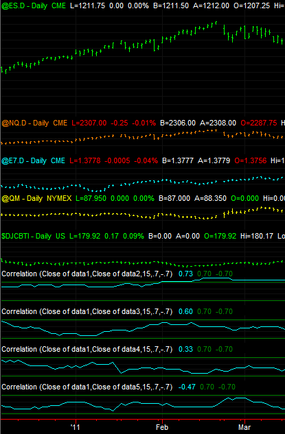
Figure 1. TradeStation price chart showing the E-mini S&P with the E-mini NASDAQ as data2, E-mini Euro as data3, E-mini crude oil as data4, and the CBOT Treasury Index as data5. The correlations between the ES and each other market are also plotted.

This collection of markets provides a second stock index, a currency, a global commodity, and an interest rate. As shown in Fig. 1, I plotted the correlation coefficient between the ES and each of the other markets. I could have also plotted the correlations between the other markets, such as the correlation between QM and E7, but I chose to limit the factors to those directly involving the ES for the sake of simplicity.

I used Adaptrade Builder to perform the genetic programming calculations. Builder allows the correlation indicators shown in Fig. 1 to be read in and included in the build process, as shown below in Fig. 2.

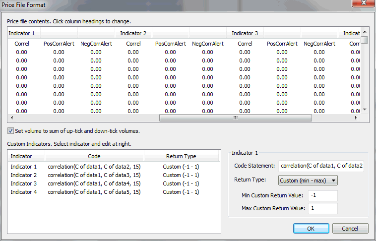
Figure 2. Including the correlation coefficients as custom indicators, read from the price file.

Each of the correlation coefficients read in from the price chart data becomes a custom indicator in Builder. The four indicators listed in the Custom Indicators table in Fig. 2 are, respectively, the correlation between the ES and the NQ, the correlation between the ES and the Euro, the correlation between the ES and mini crude oil, and the correlation between the ES and the treasury index.

All four indicators were included in the so-called build set of Builder, as shown in Fig. 3. This means the GP algorithm will consider using them in constructing strategies. I also included other indicators in the build set, including price patterns, the day of week indicator, moving averages, and the highest and lowest functions. These other indicators were included to test whether or not the correlation coefficients were better or worse than some other, common indicators. I also selected the option to make the long and short sides symmetric, which means the same logical elements will be used for entering each side of the market with the inequality operators reversed for the opposite side.

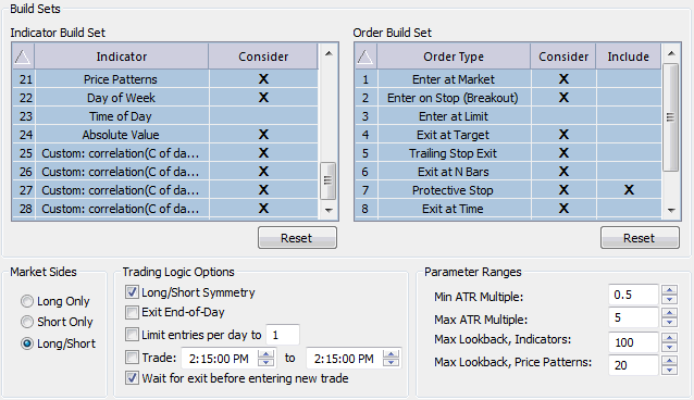
Figure 3. Including the correlation coefficients in the build set for genetic programming.

To build a strategy in Builder, it's necessary to specify a set of performance metrics. These are shown in Fig. 4. I ran 10 builds altogether. In half, I set a target for the net profit of $80,000. In the other half, I maximized the net profit. In all cases, I set targets for the correlation coefficient of the equity curve, the return/drawdown ratio, and the average bars in trades. I also set it to minimize the complexity using a relatively small weight value of 0.2. All other metrics used a weight value of 1.0, so the complexity goal was designed to give a small bias to strategies with fewer inputs.

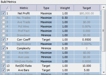
Figure 4. Build goals for genetic programming.

The time period for building strategies is shown below in Fig. 5. The ES price data consist of daily bars from February 2005 to September 2011. I set aside the most recent 25% of data for out-of-sample testing, which means the strategies were built over data from 2/2005 to 1/2010. Trading costs of $30 per round turn were used.

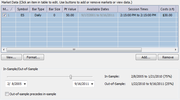
Figure 5. Market settings for the genetic programming process.

A shown in Fig. 6, the strategies were built using a population of 1000 members, evolved over 20 generations. I also used an option in Builder to re-initialize the population (basically, starting over from scratch) if the out-of-sample equity curve failed to achieve a correlation coefficient of at least 0.90 after 10 generations. In other words, I wanted the out-of-sample equity curve to be nearly straight.

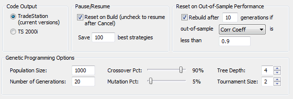
Figure 6. Various options for building the strategies using genetic programming.

Results

Ten separate builds were conducted. In nine out of 10 cases, the following entry logic was selected by the GP process:

EntCondL = correlation(C of data1, C of data3, 15) > correlation(C of data1, C of data4, 15);

EntCondS = correlation(C of data1, C of data3, 15) < correlation(C of data1, C of data4, 15);

In some strategies, the inequality operator was "<=" rather than "<" or the statement was reversed but with the same meaning (i.e., ...data4.. < ...data3...). In all nine case, though, the correlation of the ES with the Euro was compared to the correlation of the ES with crude oil.

The long entry condition (EntCondL) can be interpreted as "Entry conditions for a long trade are favored if the correlation between the ES and the Euro is stronger than the correlation between the ES and crude oil". Likewise, short entry conditions (EntCondS) are favored if the opposite holds true.

Interestingly, none of the top strategies included conditions that compared the correlation coefficient to a fixed number, such as correlation(C of data1, C of data2, 15) > 0.6.

In one case, the top strategy consisted of entry logic that did not include any of the correlation coefficients. In this case, the entry logic involved price patterns.

While the entry logic was quite consistent, the type of entry and exit orders varied somewhat. Most entries occurred on stop orders, although the stop price was calculated in different ways. A variety of exit types was used in the strategies from the different builds, including target exits, exiting after a fixed number of bars, exiting based on a separate logical condition, and so on.

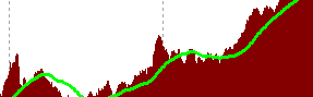
Fig. 7 shows the equity curve for the top strategy from one of the builds.

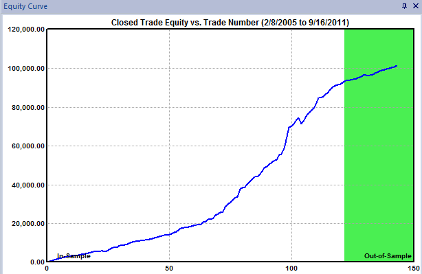
Figure 7. Closed-trade equity curve for an ES strategy using intermarket logic.

The EasyLanguage code for the strategy shown in Fig. 7 is listed below.

{
EasyLanguage Strategy Code for TradeStation
Population member: 6

Created by: Adaptrade Builder version 1.2.2.2
Created: 9/21/2011 11:10:59 AM

TradeStation code for TS 6 or newer

Price File: C:\ABStrats\ES-NQ-E7-QM-DJCBTI-10yrs.txt
Build Dates: 2/8/2005 to 1/21/2010

Project File: C:\ABStrats\AB-Corr6.gpstrat
}

{ Strategy inputs }
Inputs: NBarEn1 (17),
NBarEn2 (21),
NBarEn3 (10),
EntFr (1.4353),
NTarg1 (32),
NTarg2 (41),
TargFr (2.3421),
NMM1 (10),
NMM2 (87),
MMFr (4.6119);

{ Variables for entry and exit prices }
Var: EntPrL (0),
EntPrS (0),
TargPrL (0),
TargPrS (0),
LStop (0),
SStop (0);

{ Variables for entry and exit conditions }
Var: EntCondL (false),
EntCondS (false);

{ Entry prices }
EntPrL = L[NBarEn1] + EntFr * AbsValue(Average(H, NBarEn2) - C[NBarEn3]);
EntPrS = H[NBarEn1] - EntFr * AbsValue(Average(H, NBarEn2) - C[NBarEn3]);

{ Entry and exit conditions }
EntCondL = correlation(C of data1, C of data3, 15) > correlation(C of data1, C of data4, 15);
EntCondS = correlation(C of data1, C of data3, 15) < correlation(C of data1, C of data4, 15);

{ Entry orders }
If MarketPosition = 0 and EntCondL then begin
Buy next bar at EntPrL stop;
end;

If MarketPosition = 0 and EntCondS then begin
Sell short next bar at EntPrS stop;
end;

{ Exit orders, long trades }
If MarketPosition > 0 then begin

If BarsSinceEntry = 0 then begin
LStop = EntryPrice - MMFr * AbsValue(L[NMM1] - Lowest(L, NMM2));
end;

Sell next bar at LStop stop;

TargPrL = EntryPrice + TargFr * AbsValue(Highest(H, NTarg1) - Highest(C, NTarg2));
Sell next bar at TargPrL limit;
end;

{ Exit orders, short trades }
If MarketPosition < 0 then begin

If BarsSinceEntry = 0 then begin
SStop = EntryPrice + MMFr * AbsValue(L[NMM1] - Lowest(L, NMM2));
end;

Buy to cover next bar at SStop stop;

TargPrS = EntryPrice - TargFr * AbsValue(Highest(H, NTarg1) - Highest(C, NTarg2));
Buy to cover next bar at TargPrS limit;
end;
 

Conclusions

The fact that nine out of 10 GP builds chose to use the correlation coefficients rather than moving averages or price patterns suggests there may be some utility in intermarket analysis for trading the E-mini S&P on daily bars. More interesting is the fact that the top strategy for each build that settled on correlation coefficients used them in an unusual way. I'll leave it up to someone with a better understanding of fundamental analysis than me to determine why it might make sense to trade the long side of the ES when it's more correlated to the Euro than to crude oil. Whatever explanation one might impose to justify that logic, the fact remains that the GP process consistently found that relationship to provide more benefit than any other one it examined. It's also interesting to note that the GP process didn't find utility in the correlations between the ES and either the NQ or interest rates.

I have no doubt that some traders would be uncomfortable trading a strategy that uses logic for which they can't find a fundamental explanation. It reminds me of what happens every day on the financial news programs after the markets close. Regardless of which way the markets moved that day, the commentators and analysts look back on the day and try to explain why the markets went up, down, or sideways. However, I suspect that trying to fit an explanation to the market's behavior after-the-fact probably matters very little to all the traders who either made or lost money that day.

Copyright © 2001-2013 Breakout Futures

Copyright © 2013-2018 Adaptrade Software