|
||
|
||
|
|
|
|
Regularization and Strategy Over-Fitting by Michael R. Bryant
Regularization is a concept typically encountered in the fields of machine learning and statistical inference. In the context of systematic trading, regularization is important because it relates to over-fitting, a problem all too familiar to most systematic traders. In this article I'll show how regularization can help prevent over-fitting during strategy development. I'll also introduce a new trading strategy metric motivated by the concept of regularization and explain how it can be used to rank competing strategies to help reduce over-fitting.
When fitting a mathematical model to a set of data, a common approach is to minimize the error between the model and the data; for example, least squares curve-fitting. Regularization is based on the idea that you not only want to minimize the error between the model and the data but the complexity of the model. Methods of regularization balance degree of fit with model complexity, which leads to simpler models that still fit the data without over-fitting.
This idea is closely related to Occam's razor, which says that the simplest hypothesis that explains the data is usually the correct one. Notice that Occam's razor doesn't claim that the simplest solution is always the best one. Sometimes, a more complex solution can explain the data better than a simpler one. Occam's razor recognizes the trade-off between explanatory power and complexity and says we shouldn't increase the complexity of the solution unless it's necessary to do so.
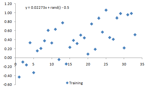
No More Complex Than Necessary To illustrate these ideas, consider the data shown below in Fig. 1. The equation displayed at the top of the chart shows how the data were generated by adding a random component to a linear equation; the "rand() - 0.5" part adds a random number between -0.5 and +0.5 to the line given by y = 0.02273x. This implies that the best model to represent the data is the linear model y = 0.02273x.
Figure 1. Example data generated by superimposing a random number between -0.5 and 0.5 to a straight line.
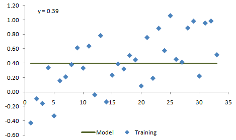
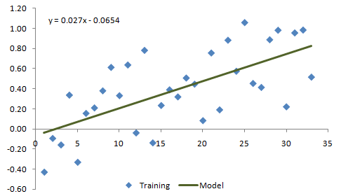
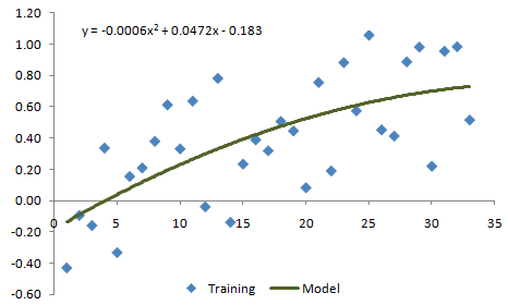
However, let's assume we were shown the data without knowing where it came from or how it was created. Our modeling approach will be to try three different models of increasing complexity: constant value, linear, and quadratic (2nd order polynomial). In each case, we'll fit the model to the data with a least-squares method. The results of this process are shown in Figs. 2 - 4.
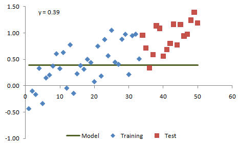
Figure 2. Example data from Fig. 1 fit with a constant value model.
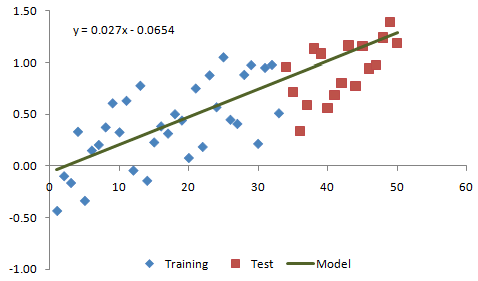
Figure 3. Example data from Fig. 1 fit with a linear model.
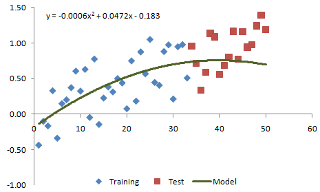
Figure 4. Example data from Fig. 1 fit with a quadratic model.
Based solely on how each of the three models appear to fit the data shown above, it's pretty clear that the linear model more accurately captures the data than the constant value model. However, it's not as clear whether the second order model is better than the linear one. So how do we determine which model fits the underlying process better?
Notice that the blue data points in Figs. 1 - 4 are labeled "Training". A common approach to model selection is to divide the data into three segments: training, test, and validation.1 The models are fit to the training data. The test data are then used to evaluate and select the model. Finally, the validation segment is used to generate an unbiased estimate of likely future performance for the selected model.
Figs. 5 - 7, respectively, show the three models extrapolated forward over additional data that have been added. The additional data points comprise the test segment. Fig. 5 shows how the constant value model performs on the test segment, where it clearly fails to fit the data very well. We can conclude that the constant value model is too simple to adequately capture the essential feature of the data, which is the up-sloping trend.
Figure 5. The constant value model is extrapolated forward to the test segment.
Figure 6. The linear model is extrapolated forward to the test segment.
Figure 7. The quadratic model is extrapolated forward to the test segment.
In Fig. 6, it's apparent that the linear model does a pretty good job of predicting the test data. The quadratic model in Fig. 7, which is starting to turn back down while the test data continues to rise, appears to be the wrong model for this data. This is an example of over-fitting. The quadratic model appears to fit the training data well but is overly complex and fails to capture the essential features of the data. Overall, the performance on the test segment clearly shows that the linear model is the best one.
How Does This Apply to Trading?
Imagine a typical trading strategy development scenario in which you start out with a fairly simple strategy. After optimizing the strategy inputs, you notice an obvious deficiency, so you decide to add another rule to improve the performance. Another round of testing leads to more additions and changes, and so on. More often than not, this leads to an over-fit strategy that fails in real time.
However, based on the example in the previous section, there's a better way to conduct this process. In particular, you would first divide your market data into three segments: training, test, and validation. Each time you make a change to the strategy that improves the results on the training data, such as adding another rule, you would run the strategy on the test segment. It's assumed that the change improves the results on the training segment; otherwise, there's no point in considering the change any further. However, if the change results in worse performance on the test segment, as we saw in moving from the linear equation to the quadratic equation in the example above, you know you've over-fit the strategy and should revert to the prior one.
It's still highly advisable to test the final strategy on the validation segment to get an unbiased estimate of likely future performance. Even though the strategy is fit to the training segment, rather than the test segment, the test segment is used to evaluate and select the strategy. As a result, the test segment also biases the results.
The essential feature of this approach is tracking the performance on the test data. As the strategy's performance on the training data continues to improve with changes to the strategy, the performance on the test segment should also improve up to the point at which the strategy becomes over-fit. Once this happens, the performance on the test segment will start to decline, which indicates that the strategy has become overly complex and over-fit. At that point, making the strategy more complex is likely to be counter-productive, and a simpler version will likely perform better on the validation segment.
Ranking Competing Strategies Using Complexity The idea of regularization lies behind the idea of using separate training and test segments to monitor strategy performance during the development phase to prevent over-fitting. There's another scenario for which the concept of regularization can help reduce the risk of over-fitting. Consider a situation in which you've developed several different strategies for the same market. Some of the strategies may be more complex, some less so.
If you've used the approach described above, you may have found that the more complex strategies performed better on the test segment, suggesting that they are not yet over-fit and may be preferred. However, how do you know if the added complexity is worth the additional performance? Occam's razor, which underlies regularization methods, says we should only add complexity if doing so is worthwhile. Even if the results on the test data suggest the results are not over-fit, there may be diminishing returns from the added complexity. It may even be the case that a simpler strategy would be less biased by the fitting process and therefore perform better on the validation segment.
This line of thinking suggests the following metric to rank competing strategies:
The Strategy Input Power (SIP) is the net profit per share or contract divided by the number of strategy inputs. This is basically the complexity-normalized net profit of the strategy. This assumes that the complexity of the strategy is represented by the number of inputs. Provided an input is used for each possible variable (i.e., no hard-coded numerical values such as dollar stop amounts or indicator look-back lengths), then the number of inputs should be a good measure of strategy complexity.
To see how this works, consider two strategies that generate the same net profit on the same market, but strategy #1 has 12 inputs whereas strategy #2 has six inputs. Strategy #2 is generating twice the profit per input as strategy #1. Because strategy #2 is simpler and generates the same net profit, we would prefer strategy #2, all else being equal. In this case, strategy #2 would have a SIP twice that of strategy #1. Similarly, if two strategies have the same number of inputs, but strategy #3 has more profit than strategy #4, strategy #3, which would have a higher SIP, would be preferred (all else being equal).
Certainly, a more practical and useful case is when neither the net profit nor the number of inputs is the same between competing strategies. In that case, the SIP can tell us which strategy is doing more with less. In general, we'd like our strategies to generate as much profit as possible with as few inputs as possible, which means a higher SIP is preferred over a lower one.
Another way to view the SIP is as the efficiency of the strategy logic. The more "efficient" the logic is at generating profits, the more profit will be generated per input. By ranking competing strategies by the SIP, the more efficient strategies will be ranked higher.
Summary Occam's razor suggests that a model should not be any more complex than necessary. Regularization methods formalize this idea to help prevent over-fitting. Using training and test segments to guide the selection of strategies during the strategy development process is a regularization technique that can be used to help avoid over-fit trading strategies. The Strategy Input Power (SIP) metric can be used to compare and rank competing strategies applied to the same market. As with regularization, preferring strategies with a higher SIP may help prevent over-fitting and therefore increase the chances of positive results going forward.
Reference
Mike Bryant Adaptrade Software
*This article appeared in the May 2012 issue of the Adaptrade Software newsletter.
|
If you'd like to be informed of new developments, news, and special offers from Adaptrade Software, please join our email list. Thank you.
For Email Marketing you can trust
|
|||||||||||||
|
|
|
|
|||||||||||||
Copyright (c) 2004-2019 Adaptrade Software. All rights reserved.