Preventing Over-Fitting During Optimization

by Michael R. Bryant

Over-fitting occurs when a trading strategy is optimized so that it fits the data used in the optimization well but doesn't fit any other data very well. An over-fit strategy doesn't generalize well to new data. Any part of the data that can be traded profitably can be considered the signal, while everything else can be considered noise. Over-fitting is fitting the noise, rather than the signal.¹

Over-fitting can result from over-optimization. By definition, optimization fits the strategy to the data used in the optimization. There is nothing inherently wrong with this. As Aronson points out, data mining is based on a sound premise.² Generally speaking, the best observed result is better than a randomly chosen result, and evaluating more options generally leads to better results. However, optimizing beyond the point at which the signal is fit can lead to fitting the noise and therefore result in over-fitting. This is over-optimization.

It might be possible to avoid over-fitting simply by limiting the optimization. However, this is an imprecise solution to a complex problem. How much optimization is too much? At what point do you stop? How do you know when you've gone too far? This article describes a more direct approach based on monitoring the optimization process.

Detecting Over-Fitting

If we want to avoid over-fitting by monitoring the optimization process, we need a way to detect when over-fitting occurs. An unbiased test of the optimized results can be used for this purpose. The data over which the optimization is performed is called the training segment. The test segment is some portion of the data reserved for monitoring. The basic idea, then, is to perform the optimization on the training segment and monitor it by evaluating the results on the test segment.

Ideally, we'd like the results on the test segment to be similar to the results on the training segment. If each step of the optimization improves the results on the training segment, we'd like the results on the test segment to improve as well. If, however, the results on the training segment continue to improve during the optimization process, but the results on the test segment stop improving or start to decline, it suggests the results are being over-fit.

Why do declining results on the test segment indicate over-fitting? The optimization process guarantees that the results on the training segment will improve or at least not get worse. This is how optimization works. It selects the results that are best on the training segment. If the optimized strategy is then tested on data not used in the optimization -- the test segment -- and the results there are positive, it suggests that the optimization is correctly fitting the signal, rather than the noise.*

If it wasn't fitting the signal, but was fitting the noise instead, it's unlikely that the results would hold up on the test segment. That's because the noise component of the price data is random by definition, which means it's unlikely to repeat in the test segment. If the noise component is different in the test segment, a strategy fit to the noise of the training segment is unlikely to do well in the test segment. Therefore, an optimized strategy that performs well on the training segment but fails on the test segment has probably been fit to the noise of the training segment and is therefore over-fit.

However, one other possibility should be considered. As Bandy discusses, financial markets tend to be non-stationary.³ This means the statistical properties tend to vary from one region of the data to another. If the statistical properties relevant to the trading strategy vary from the training segment to the test segment, the optimization could fit the signal correctly yet the results on the test segment could be poor. For this reason, to asses over-fitting using this approach, it's important to look for a decline in results on the test segment, rather than poor results from the start. In summary, then, over-fitting will be indicated by results that are initially good on the test segment but start to decline as the results on the training segment continue to improve. In other words, we're looking for a divergence in results between training and test.

Rules for Monitoring Optimization

Two sets of rules have been added to Adaptrade Builder to monitor the optimization process and detect over-fitting. Adaptrade Builder uses a genetic programming (GP) process to construct trading strategies. The GP process is a type of optimization that evolves a population of strategies over successive generations. Each strategy is back-tested on the selected market data to determine a "fitness" value for the strategy. The optimization process maximizes the fitness.

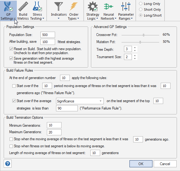
As shown below in Fig. 1, one set of rules is referred to as the Build Failure Rules. These rules are designed to restart the build process if the results on the test segment are not acceptable. In practice, this could be due to (1) poor fit in general, (2) non-stationary conditions, or (3) over-fitting on the training segment.

Figure 1. Rules for monitoring optimization during strategy building in Adaptrade Builder.

There are two optional rules, either of which or both can be selected. The selected rules are applied once during the build/optimization process at the end of the specified generation. The two rules are designed as a check on the validity of the build process. If it passes the check, the process continues until completion. If not, the optimization is halted, and the process is restarted.

The first rule ("Fitness Failure Rule") computes the average fitness of the strategies in the population, where the fitness is calculated on the test segment. It then takes a moving average of this population-average fitness. If the moving average of fitness is less than it was N generations ago, it indicates that the fitness on the test segment is declining. The length of the moving average and the value of N are user inputs. Since this check is generally performed early in the build process, a drop in the fitness on the test segment indicates a failure of the build process. As noted above, this could be due to over-fitting or possibly other causes.

The second Build Failure Rule ("Performance Failure Rule") calculates an average of the specified performance metric on the test segment over the fittest N strategies in the population. If this average value is less than a specified threshold, it indicates that the performance on the test segment is unacceptable, and the build process is considered to have failed. The build process is then restarted. For example, the rule might be to start over if the average net return on the test segment of the top 5 strategies is less than 20%.

The two different Build Failure Rules provide different ways to identify when the build process is not working. Selecting both rules means the build process will be restarted at the end of the specified generation if either rule is true at that point.

The rules shown under Build Termination Options in the bottom part of Fig. 1 more directly target over-fitting. The basic idea is that the build failure rules are applied first. If the build process passes these checks, the optimization continues until the minimum number of generations specified under Build Termination Options is reached. At that point, the build termination rules are applied at the end of each generation until either the maximum number of generations is reached or one of the termination rules applies.

Both build termination rules are based on the average population fitness calculated on the test segment. The first rule follows the same form as the Fitness Failure Rule: the moving average of the population-average fitness on the test segment is compared to its value N generations ago. If the moving average is less than it was previously, the build process is stopped due to the decline in fitness on the test segment. As discussed above, this indicates over-fitting when it happens in the presence of increasing fitness on the training segment, assuming the results on the test segment were initially positive. The latter is assured by the proper use of the Build Failure Rules.

The second build termination rule compares the population-average fitness on the test segment with its moving average. If the fitness is below its moving average, the build process is terminated. This is just a different way to detect a decline in the fitness on the test segment. Either one or both of the build termination rules can be selected. If both are selected, the build process will be stopped if either one applies.

It should be noted that over-fitting is not the only condition that can trigger the build termination rules. In some cases, no further improvement in the results may be possible, even on the training segment. This just means the optimization algorithm has found a maximum, and additional generations of the GP algorithm are unlikely to improve the results. In this case, the results on the training segment will peak, and, provided the strategy is not over-fit, the results on the test segment will peak at about the same time.

Optimization Monitoring in Action

To illustrate these concepts, consider an example build project for the E-mini Russell 2000 futures (symbol TF). Daily bars of day session data for TF.D were obtained from TradeStation for the date range 11/7/2001 to 8/27/2015. The training segment was set to 11/7/2001 to 9/14/2010 and the test segment to 9/15/2010 to 11/30/2012. The remaining data were set aside for validation. Trading costs of $25 per round turn were used.

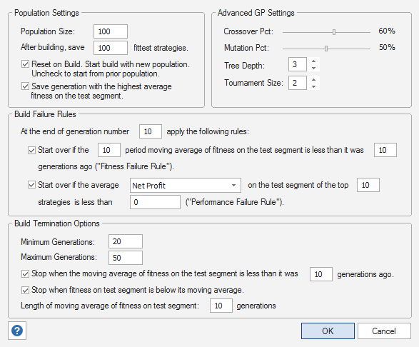
As shown below in Fig. 2, the build failure rules were set to apply at the end of generation 10. The performance failure rule was set to restart the build if the average net profit of the top 10 strategies on the test segment was negative. The minimum number of generations was set to 20 with a maximum of 50 generations. Both build termination rules were selected using the default settings.

 Figure 2. Settings for example based on the mini Russell 2000 futures.

A short video showing how the build process proceeded is shown below. Initially, the average net profit on the test segment was negative. However, by the end of generation 10, the results were positive, which allowed it to pass the build failure checks. After 20 generations, the build termination rules were applied at the end of each generation. At the end of generation 21, the average fitness on the test segment crossed below its moving average, triggering the second build termination rule, which stopped the build.

An expanded picture of the Build Termination Tracking plot from the Build/Eval Process window is shown below in Fig. 3 at the end of the build process. As shown in the figure, the fitness on both the training and test segments increased as the build process proceeded until generation 15, which was the peak of the fitness on the test segment. Although the fitness on the training segment continued to improve, the fitness on the test segment started to decline, indicating over-fitting. It took several more generations for the fitness on the test segment to cross below its moving average, which triggered the build termination rule to stop the build. The aforementioned divergence between the training and test results is clearly visible at generation 21.

Figure 3. The build termination tracking plot depicts the build termination rules selected on the GP Settings window. The blue line is the fitness on the training segment. The red line is the fitness on the test segment, and the green line is the moving average of the red line.

Notice that there is a rule, which was selected on the GP Settings window (Fig. 2), that saves the generation with the highest fitness on the test segment. This ensures that even if it takes a few generations to detect the decline in fitness on the test segment, the best results prior to over-fitting will be recorded.

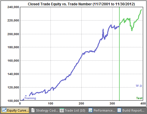
As noted above, data was set aside following the test segment to use in validation testing. We can test one of the top strategies to see if it holds up on data not used during the build process. Fig. 4 shows the equity curve for one of the top strategies over the training and test segment, excluding the validation data. This in-sample equity curve shows positive results on the test segment, as expected.

 Figure 4. Equity curve for an E-mini Russell 2000 strategy on (in-sample) data used in the build process.

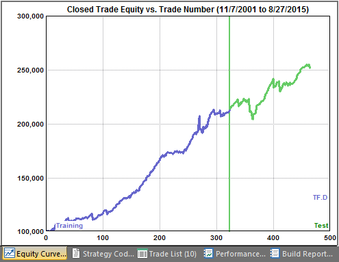
If the reserved data from the end of the test segment through 8/27/2015 are added and the strategy is re-evaluated, the equity curve shown below in Fig. 5 is produced.

Figure 5. Equity curve for an E-mini Russell 2000 strategy on (out-of-sample) data reserved for validation testing.

As shown above, the strategy holds up well out-of-sample. Of course, just because the strategy was not over-fit does not mean it will necessarily hold up well out-of-sample or going forward in real time. As discussed above, the financial markets tend to be non-stationary, which means they can change over time, invalidating a strategy that was previously profitable. Conversely, the fact that a strategy does not perform well out-of-sample does not necessarily mean it was over-fit. It might fail out-of-sample due to non-stationary conditions or because of data mining bias. The latter can be tested for in Adaptrade Builder by running a significance test that takes into account the GP process and the number of strategies generated during the build.

Conclusions

Strategy traders not only have to contend with market risk but with the risks inherent in developing trading strategies. Over-fitting a trading strategy during optimization is one of the risks in strategy development. This article demonstrated rules built into the Adaptrade Builder strategy building software that monitor the optimization process to detect and prevent over-fitting. Having these rules can help increase the reliability of strategies generated using an automated tool like Builder.

While monitoring the optimization process can be an effective way to prevent over-fitting, it's not the only approach. As discussed in a prior article, a certain amount of robustness can be built-in to strategies using a stress testing approach in which key inputs and other variables are varied during the build process and the results are evaluated across all data sets. Another approach is to select strategies during the optimization process that are less likely to be over-fit by choosing optimization goals that relate to strategy robustness, such as correlation coefficient of the equity curve, complexity, and the number of trades. The user's guide for Builder has a more complete discussion of this approach in the Usage Topics chapter.

Optimization monitoring rules, such as those discussed here, combined with stress testing methods, effective optimization/build metrics, and significance testing can help maximize a trader's confidence in the strategies generated from optimization. Add to this list out-of-sample/validation testing and/or real-time tracking, and there should be little doubt about the quality of a trading strategy prior to real-time trading.

Good luck with your trading.

Mike Bryant

Adaptrade Software

* It only "suggests" the optimization is fitting the signal. We can't be confident this is true without performing a significance test to determine if the results are good mostly due to chance.

_____________________

This article appeared in the August 2015 issue of the Adaptrade Software newsletter.

HYPOTHETICAL OR SIMULATED PERFORMANCE RESULTS HAVE CERTAIN INHERENT LIMITATIONS. UNLIKE AN ACTUAL PERFORMANCE RECORD, SIMULATED RESULTS DO NOT REPRESENT ACTUAL TRADING. ALSO, SINCE THE TRADES HAVE NOT ACTUALLY BEEN EXECUTED, THE RESULTS MAY HAVE UNDER- OR OVER-COMPENSATED FOR THE IMPACT, IF ANY, OF CERTAIN MARKET FACTORS, SUCH AS LACK OF LIQUIDITY. SIMULATED TRADING PROGRAMS IN GENERAL ARE ALSO SUBJECT TO THE FACT THAT THEY ARE DESIGNED WITH THE BENEFIT OF HINDSIGHT. NO REPRESENTATION IS BEING MADE THAT ANY ACCOUNT WILL OR IS LIKELY TO ACHIEVE PROFITS OR LOSSES SIMILAR TO THOSE SHOWN.

If you'd like to be informed of new developments, news, and special offers from Adaptrade Software, please join our email list. Thank you.