|
||
|
||
|
|
|
|
Building Trading Strategies Using Inter-Market Logic by Michael R. Bryant
One way to classify technical trading approaches is according to whether the trading logic is based solely on the symbol being traded or on multiple symbols. Proponents of approaches based on a single symbol argue that all information that affects how a symbol trades is reflected in the symbol's price and volume (and open interest for futures). This is based on the idea that market participants have access to all relevant information, which they consider when buying and selling the symbol. As a result, the symbol's price and volume incorporate all information that the market deems important. If this is true, including data from other markets and sources would not only be unnecessary but potentially counter-productive as it would add additional noise without any added signal.
Others note that since markets are influenced by a variety of related markets and fundamental data, these other symbols should be included in the logic for the market being traded. They point out that certain markets are known to be correlated and that some markets seem to lead or lag other ones. Another argument in favor of this approach is that adding other, related symbols to the logic for the primary symbol provides confirmation and can reduce the effects of noise in the primary symbol's data.
Basing trading decisions for one symbol on other symbols in addition to the tradable is typically called inter-market analysis. For example, you might look for divergences between the NASDAQ 100 and the E-mini S&P 500 to decide when to enter a trade in the latter. Or you might look for trends in the dollar index when making decisions about crude oil.
Adaptrade Builder is primarily intended for developing trading strategies based on signals from the market being traded. However, the custom indicator feature in Builder allows it to incorporate other symbols into the entry and exit logic, provided those symbols have the same bar size as the primary symbol. This article shows how recent improvements to the custom indicator feature make it possible to incorporate price data from several additional symbols into the entry and exit logic by defining the individual prices of the secondary symbols as custom indicators. In addition, numerical testing results show that this can lead to better out-of-sample results.
Prices as Custom Indicators Adaptrade Builder constructs trading strategies by combining indicators, price patterns, and other trading logic options so that the resulting strategies meet the user's performance specifications and requirements. Typically, the logical conditions for entry and exit consist primarily of indicators that are built into the program.
The custom indicator feature in Builder was developed to allow the user to include indicators in the build process that are not part of the built-in set. To include a custom indicator, you would add an extra column of data to the price file for each custom indicator. The extra column of data consists of the indicator values for each bar of price data. For example, if you have a proprietary trend indicator and you're building a strategy for Apple stock, you would plot the trend indicator on the chart for Apple and save the resulting chart data. In some trading platforms, such as TradeStation and MultiCharts, this allows you to save both the price data for Apple as well as the indicator values. The latter are saved in a separate column in the same file. If your platform doesn't allow this, you would use a spreadsheet to add an extra column to the file of price data for the custom indicator values.
When you use the resulting file of price data in Builder, you can identify the extra column as containing the custom indicator values. The program can then include that data in the build process. Builder also allows you to assign a code function name to the indicator. This name is substituted into the code that Builder generates whenever the custom indicator values are used. It's up to the user to make sure this function is available when the strategy is run in the trading platform so that it will return the same indicator values that were provided in the price file in the custom indicator column.
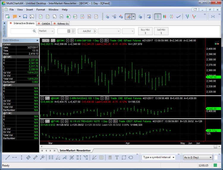
To see how this process works for including other symbols in the build process, consider the chart window shown below in Fig. 1, which was created in MultiCharts 10. As shown in the figure, the main chart ("data1" in the terminology of the EasyLanguage scripting language) plots daily bars of the E-mini S&P 500 futures (symbol @ES#C, obtained from IQFeed). Two additional sub-charts have been added for the mini NASDAQ 100 (@NQ#C) and 10-year Treasury Notes (@TY#C), which are referred to in EasyLanguage as data2 and data3, respectively.
Figure 1. Price chart consisting of daily bars of the E-mini S&P 500 futures as the primary symbol (data1) with the mini NASDAQ 100 and 10-year Treasury Notes plotted as data2 and data3, respectively.
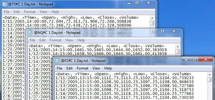
MultiCharts doesn't allow all three symbols to be saved to the same file, but the chart data for each symbol can be saved separately, as shown below in Fig. 2, where each price file has been saved as a text (.txt) file and opened in NotePad. Each price file consists of the date, time, open, high, low, close, and volume for each trading day from 1/11/2005 to 4/21/2017.
Figure 2. Raw price data for the three symbols saved from the chart shown in Fig. 1
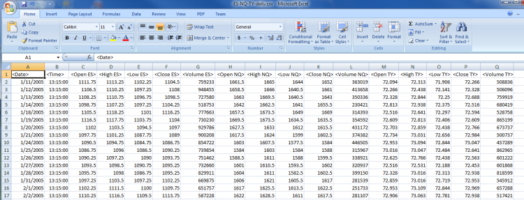
The next step is to combine the three price files into one file using Excel, as shown in Fig. 3. This is just a matter of opening each text file in Excel and copying the columns, making sure the dates match up. The only caveat is that not all symbols trade on all the same days. In this case, Treasury Notes didn't trade on several government holidays where the stock index futures did. As a result, there were some date mismatches that had to be manually corrected. The best way to handle this is to manually add a row for each missing date, where all the prices on the missing date are set to the close of the prior date and the volume is set to zero.
Figure 3. The price data for multiple symbols can be combined in a spreadsheet.
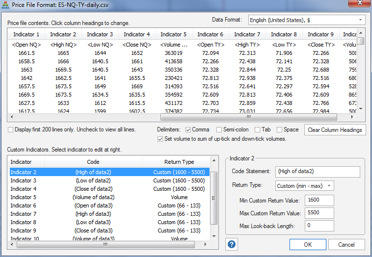
Once the individual price files are combined, the spreadsheet can be saved as a comma-delimited text file (extension .csv). To use this file in Builder, it is first added to the symbol library, which brings up the Price File Format window, as shown below in Fig. 4. This is where the custom indicators are defined.
Figure 4. Custom indicators are defined on the Price File Format window.
Each column that contains a price or volume from one of the secondary data series can be identified as a custom indicator by clicking on the column heading and selecting "Indicator" from the pop-up menu. The code statement and return type for each indicator are entered in the right-hand box below the table of prices. For example, in the table of custom indicators in the lower left-hand side of Fig. 4, indicator 2 has been selected. The strategy code -- in this case, EasyLanguage code -- has been set to "(High of data2)" in the right-hand box. This indicates that the data in the column labeled as "Indicator 2" consists of the high of data2, which is the mini NASDAQ 100. If this indicator is selected by Builder to be used in a strategy, "(High of data2)" will appear in the strategy code. When a strategy that contains this custom indicator is run in the trading platform, it will be the user's responsibility to make sure that data2 is set to the mini NASDAQ 100.
Also note from Fig. 4 that the return type for Indicator 2 has been set to "Custom (min - max)", which means this indicator returns a value in the range given by the min and max entries: 1600 to 5500. From the table of custom indicators, it can be seen that the return ranges for all the prices for the mini NASDAQ 100 have been set to the same range. This is how the program knows that, for example, "Low of data2" can be compared to "Close of data2". Likewise, a different custom return range has been entered for indicators six through nine, which represent 10-year Treasury Notes. Using a different return range prevents comparisons between data2 and data3.
The look-back length for the custom indicators has been set to zero since price data do not require a look-back period. Lastly, the volume columns for the NASDAQ 100 and Treasury Notes have been set to the return type "Volume", which is one of the predefined return types. All predefined return types refer to the primary data series. By setting the volume data for the secondary series to the same type as the volume for the primary series, we're allowing comparisons between volumes for the different symbols. For example, we might want to allow something like "(Volume of data2) crosses above Volume." If you didn't want to allow this type of comparison, custom return types could be used for the volume indicators for data2 and data3.
An Example of Auto-Generated Inter-Market Logic To illustrate the types of strategy logic that this approach can generate, the price data described above were used to generate several strategies for daily bars of the E-mini S&P 500 futures. All ten custom indicators were included in the build (four prices plus volume for two symbols) except that the volume indicators were removed from the build set for some runs in order to give more emphasis to the price data. The build metrics used to define the fitness for evolving the population of strategies are shown below. The code examples that follow were taken from strategies in the Top Strategies population.
Build Objectives
A fixed position size of one contract was used, and commission and slippage costs of $25 per round turn were deducted from each trade. The population size was set to 500 with 60 generations. Some runs were manually stopped prior to the 60th generation. The data was split 60% training/40% out-of-sample; since no build failure or termination rules were used, the second segment was out-of-sample. EasyLanguage (TradeStation/MultiCharts) was selected as the code type. Default values were used for the remaining settings.
In the examples that follow, the results were positive on both the training and out-of-samples periods. The next section will look at profitability directly.
Here's an example of a long entry condition that compares the volume of the NQ to the volume of the ES.
{ Entry and exit conditions }
The long entry condition (EntCondL) can be written as Highest(Lowest(Volume, N1), NL2)[ShiftL1] > Volume of data2. In other words, a long entry order is placed (a stop order in this case) if the highest of the lowest volume of the ES of ShiftL1 bars ago is greater than the volume of the NQ.
The following code shows a strategy that uses different prices of data2 (NQ) in a long exit condition (variable ExCondL) involving several different transformations of the NQ prices:
{ Entry and exit conditions } The long exit condition can be written as AdaptiveVMA(Highest(Open of data2, NL3), NL4, NL5, XL1) < TriAverage(Average((Low of data2)[ShiftL1], NL6), NL7). In other words, it's comparing a smoothed version of the highest of the open of NQ to a smoothed version of the low of NQ, shifted. If the first is below the second, it exits next bar at market.
In the example below, the high of TY (Treasury Notes, data3) is compared directly to a doubly-smoothed version of the low of TY as a long exit condition (VarL1 >= VarL4). This code also illustrates how price (in this case, Low of data3) can be compared directly to a fixed value (i.e., VarS1 crosses below XS1). The fixed value, XS1, is selected by the program from the custom return range entered on the Price File Format window. If the low of TY crosses below this value, a short entry order will be placed.
{ Entry and exit conditions }
The final example illustrates a compound entry condition involving both the primary symbol and data3 (TY):
{ Entry and exit conditions }
Notice that CondS1 is true if the day-of-the-week (DayOfWeek(date)) is equal to NS1, which happens to be 2, representing Tuesday. The condition variable CondS2 compares the open of TY to a smoothed version of the low of TY (i.e., smoothed by the AdaptiveZLT function). The short entry condition (variable EntCondS) is equal to "CondS1 = CondS2". This means that a short entry order will be placed (in this case, a stop order) if both CondS1 and CondS2 are true at the same time or they're both false at the same time. In other words, if CondS2 (open of TY below the smoothed low of TY) is true on a Tuesday or if CondS2 is false on any day other than Tuesday, the short entry stop order will be placed.
Out-of-Sample Profitability As the preceding code examples demonstrate, secondary symbols can be incorporated into the build process in a meaningful way with considerable variety. A remaining question is whether doing so is generally better than basing the trading logic solely on the primary symbol. To address this question, the build process was repeated 20 times using all three symbols, as in the examples above, and another 20 times with only the primary symbol (E-mini S&P 500).
For each run, a population size of 1000 strategies with 20 generations was used. All other settings were the same as described above. To measure the success of each build, two results were recorded: the fraction of strategies profitable on the training segment that were also profitable out-of-sample, and the average out-of-sample net profit of strategies that were profitable on the training segment. Both results were intended to measure how well strategies held up out-of-sample. In addition, the average complexity of the strategies that were profitable on the training segment was recorded. The Top Strategies population was not used for these tests.
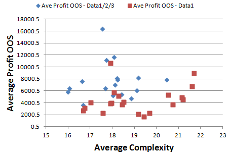
The more visually obvious result is shown in Fig. 5, below, which plots the average out-of-sample net profit of strategies that were profitable on the training segment. The blue diamonds represent the average results using all three symbols (ES, NQ, TY), and the red squares represent the results using only the primary symbol (ES). Each data point represents the average population results from one build.
Figure 5. The average out-of-sample (OOS) net profit of strategies that were profitable on the training segment versus average complexity. The populations built with all three symbols (blue diamonds) had higher average OOS profits and lower complexity compared to including only the primary symbol (red squares).
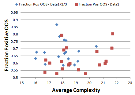
The diamonds tend to be clustered higher on the graph than the squares and appear to have more points at lower average complexity values. Similar, though less obvious, results are seen when plotting the fraction of strategies in the population profitable on the training segment that were profitable out-of-sample, as shown below in Fig. 6.
Figure 6. The fraction of strategies profitable on the training segment that were profitable out-of-sample versus average complexity. Blue diamonds represent populations built using all three symbols; red squares represent populations based only on the primary symbol.
To determine if the average population results were statistically different between the two test groups, a two-tailed t test was performed for each of the three measurements: average out-of-sample profit, fraction of profitable out-of-sample results, and average complexity. Based on a 95% confidence level (i.e., a probability threshold of 0.05), all three results were significantly different when building with all three symbols as compared to just the ES. The results are summarized in the table below. Statistical significance is indicated by the Probability values below 0.05.
The average out-of-sample (OOS) net profit of $7400 for populations built using all three symbols was significantly higher than the OOS net profit of $4500 for populations built with only the primary symbol. 69% of the strategies for which the results were profitable on the training segment were profitable out-of-sample in populations built with all three symbols compared to 62% of strategies for populations built with only the primary symbol. The average complexity of 17.6 was significantly less for populations built with all three symbols than the average complexity of 19.0 for populations built with only the primary symbol. For both test groups, the fraction of the population that was profitable in the training segment after 20 generations (i.e., the end of the build) was approximately 90% (not significantly different between the two groups).
Discussion Considering the complex interactions among markets, it's not surprising that some traders prefer approaches that include more than one symbol in the logical conditions for entry and exit. It was shown in this article that such inter-market approaches can be implemented effectively in Adaptrade Builder with a little extra work to prepare the data. By utilizing the custom indicator feature of Builder, price and volume data from other symbols can be included in a wide variety of logical conditions for trade entry and exit.
For the E-mini S&P 500 futures example considered here, testing suggests that the results of including the mini NASDAQ 100 and 10-Year Treasury Note futures in the build process results in improved out-of-sample performance. Although the reason for this is not clear, it may be due to the secondary symbol confirming the primary symbol, such as an entry condition based on the secondary symbol with an entry on a stop order to confirm.
Some types of expected inter-market logic were not seen in the results, such as inter-market divergences. However, the rule-building engine of Builder is capable of expressing this type of logic, so it may simply be that other logical conditions had more merit in the example presented.
One interesting result was that the complexity of strategies built using all three symbols was significantly less than the complexity of strategies built with only the primary symbol. In Builder, complexity is defined as the total number of strategy inputs, most of which are parameters for entry and exit conditions. In part, this result may be related to the build objective to minimize complexity. All other things being equal, the complexity objective means the less complex strategy will rank higher. The fact that, on average, higher out-of-sample net profit was seen in strategies with less complexity tends to refute the idea that adding additional symbols means adding more noise with no additional signal. In fact, the opposite appears to be true for the example presented.
Another aspect of the complexity data is that, while the complexity was significantly lower for the inter-market strategies, the difference amounted to less than two strategy inputs on average. Because the build objectives were kept very simple, involving just net profit and complexity, most of the fitness value was due to the build objectives. As a result, the build objective for complexity had the effect of evolving strategies that were no more complex than necessary to meet the build objectives. The resulting strategies had a relatively narrow range of complexity values. In fact, the standard deviation of the average complexity values across the 20 builds was less than 10% (not shown) for both test groups. This result suggests that there is a "correct" level of complexity for these strategies. Rather than simpler necessarily being better, the strategies require a certain level of complexity to achieve the performance requirements.
However, the level of complexity required to achieve the performance requirements differed slightly between the two test groups. Specifically, the strategies that result from including the secondary symbols in the build process appear to utilize the data more effectively so that they require slightly fewer inputs to achieve the same result. In this sense, simpler is in fact better since the strategies with fewer inputs -- the ones that utilize the additional symbols -- produced better out-of-sample results.
While it may be difficult to generalize these results to other markets and combinations of symbols, the results suggest that building with inter-market logic may be worth considering for your next strategy project.
Good luck with your trading.
Mike Bryant Adaptrade Software _____________________
The features described in this article are available in Adaptrade Builder version 2.2.0 and later.
This article appeared in the April 2017 issue of the Adaptrade Software newsletter.
HYPOTHETICAL OR SIMULATED PERFORMANCE RESULTS HAVE CERTAIN INHERENT LIMITATIONS. UNLIKE AN ACTUAL PERFORMANCE RECORD, SIMULATED RESULTS DO NOT REPRESENT ACTUAL TRADING. ALSO, SINCE THE TRADES HAVE NOT ACTUALLY BEEN EXECUTED, THE RESULTS MAY HAVE UNDER- OR OVER-COMPENSATED FOR THE IMPACT, IF ANY, OF CERTAIN MARKET FACTORS, SUCH AS LACK OF LIQUIDITY. SIMULATED TRADING PROGRAMS IN GENERAL ARE ALSO SUBJECT TO THE FACT THAT THEY ARE DESIGNED WITH THE BENEFIT OF HINDSIGHT. NO REPRESENTATION IS BEING MADE THAT ANY ACCOUNT WILL OR IS LIKELY TO ACHIEVE PROFITS OR LOSSES SIMILAR TO THOSE SHOWN. |
If you'd like to be informed of new developments, news, and special offers from Adaptrade Software, please join our email list. Thank you.
For Email Marketing you can trust
|
|||||||||||||||||||||||||||||||||||||
|
|
|
|
|||||||||||||||||||||||||||||||||||||
Copyright (c) 2004-2019 Adaptrade Software. All rights reserved.